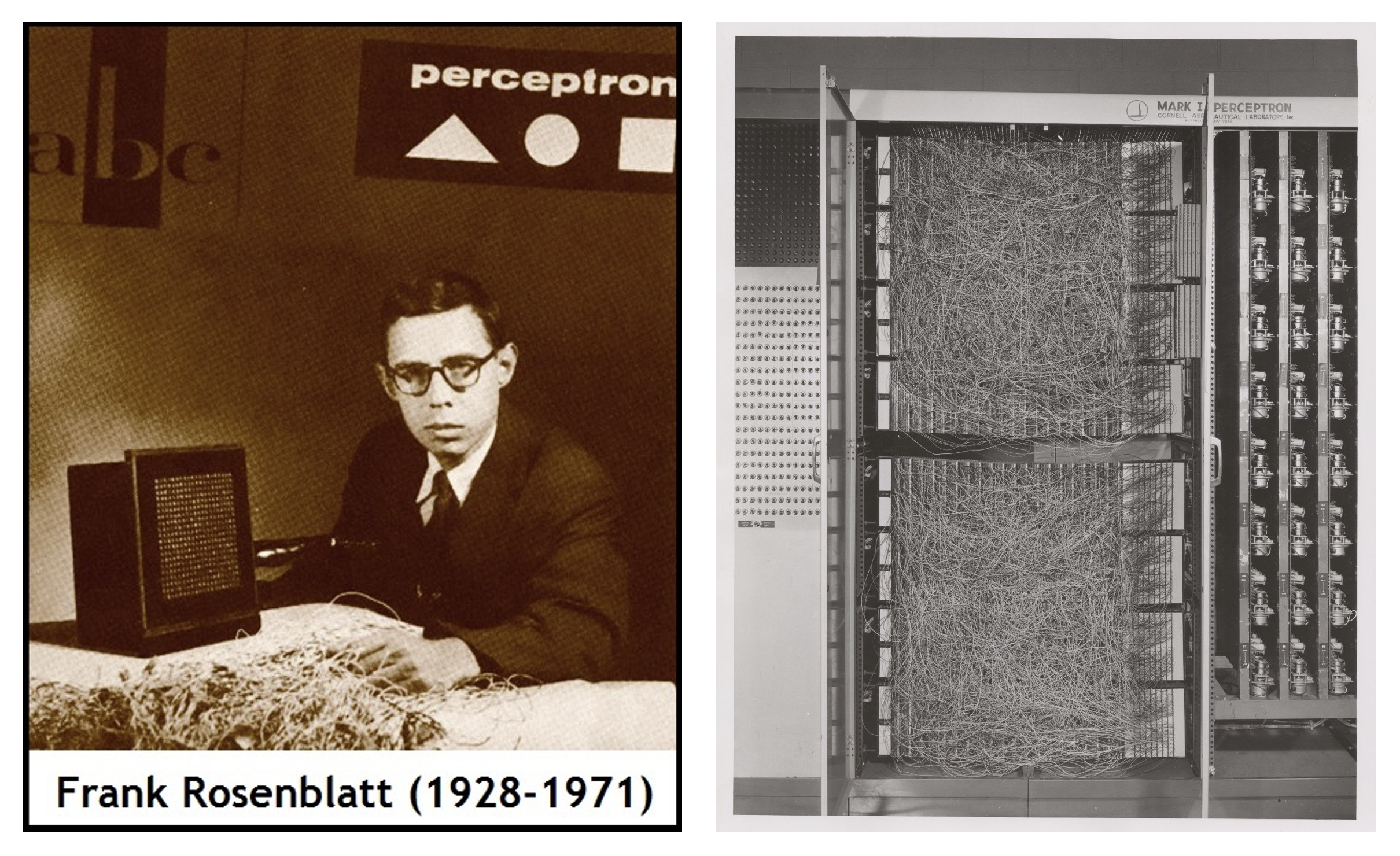
History
Proceptron classifier is viewed as the foundation and building block of artificial neural network. For a historical introduction, see the figures below.

Suppose we are solving a binary classification problem with \(p\) feature variables. As discussed before, it can be represented as
\[ \hat{y} = \text{Sign}( \textbf{w}^{\top} \textbf{x} + w_0 ) \]
where \(\textbf{w} = (w_1, w_2, \dots, w_p)^{\top}\), and \(\textbf{x} = (x_1, x_2, \dots, x_p)^{\top}\). Different from before, here we represent the weighted sum of \(p\) feature variables, \(w_1x_1+ \dots + w_px_p\), as the inner (dot) product of two vectors, i.e. \(\textbf{w} \cdot \textbf{x} = \textbf{w}^{\top} \textbf{x}\).
- Note: In order to understand proceptron algorithm, we need some basic knowledge about vector and its operations. If you are not familiar with it or need to refresh it, read about vector, operators, inner product before start reading the next.
The perceptron algorithm is about finding a set of reasonable weights. The key term here, “reasonable,” is easy to understand—it refers to a set of weights that can deliver good predictive performance. The core issue is how to find them.
- Brute-force idea: try all possible weight values and record the corresponding model performance, such as accuracy, and then choose the weights that yield the highest accuracy as the final model parameters.
However, this idea is clearly not ideal. Even if we only have two feature variables, this would still not be a simple task. A smarter approach is to do it this way: we start with an initial guess for the weight values, and then gradually approach the most reasonable weights through some iterative mechanism. This mechanism is called the perceptron algorithm. Next, let’s dive into learning this magical mechanism—the perceptron algorithm.
Next, the logic goes like this:
- Further explore the geometric properties of linear classifiers
- Use geometry to understand how this algorithm works.
