Geometry of Linear Classifiers
Note: From now, we will temporarily ignore the bias term, \(w_0\), or assume it as \(0\). It will not influence our final conclusion. No worries. So, the basic classifier is represented as \(y = \text{Sign}(\textbf{w}^{\top}\textbf{x})\)
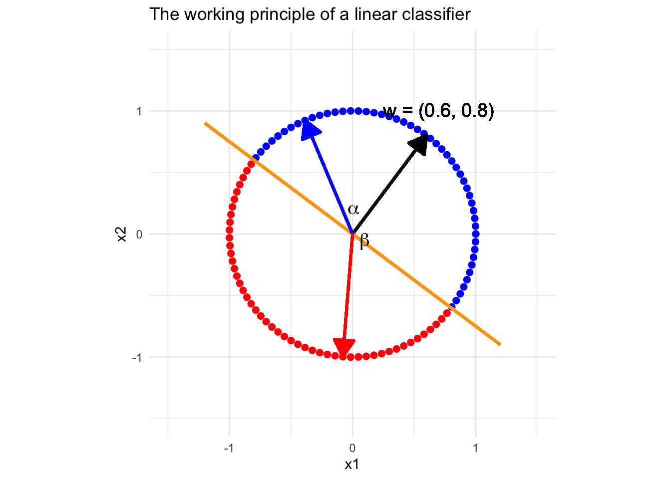
Previously, we explored the geometric understanding of linear classifiers, which is that the classifier determines a linear decision boundary. Next, let’s understand a linear classifier from another view of geometry. Suppose we have a classifier with two feature variables, \(x_1\) and \(x_2\), and the “reasonable” weight vector is \(\textbf{w} = (0.6, 0.8)^{\top}\). Look at the conceptual plot below.
It is easy to see that all the vectors (points) in blue form a sharp angle with the weights vector (black). By the property of inner product, (read about inner product) for any point \(\textcolor{blue}{\textbf{x}} = (\textcolor{blue}{x_1},\textcolor{blue}{x_2})^{\top}\) standing on the direction pointed by the blue arrow, \(\textbf{w}^{\top}\textcolor{blue}{\textbf{x}} \propto \cos(\alpha) > 0\), i.e. all the cases on this direction will be classify as positive. On the contrary, all the vectors (points) in blue form a obtuse angle with the weights vector, and then \(\textbf{w}^{\top}\textcolor{red}{\textbf{x}} \propto \cos(\beta) < 0\), i.e. all the points standing on the direction pointed by a red vector will be classified as negative. With this observation, we can easily understand how does a “reasonable” linear classifier work.
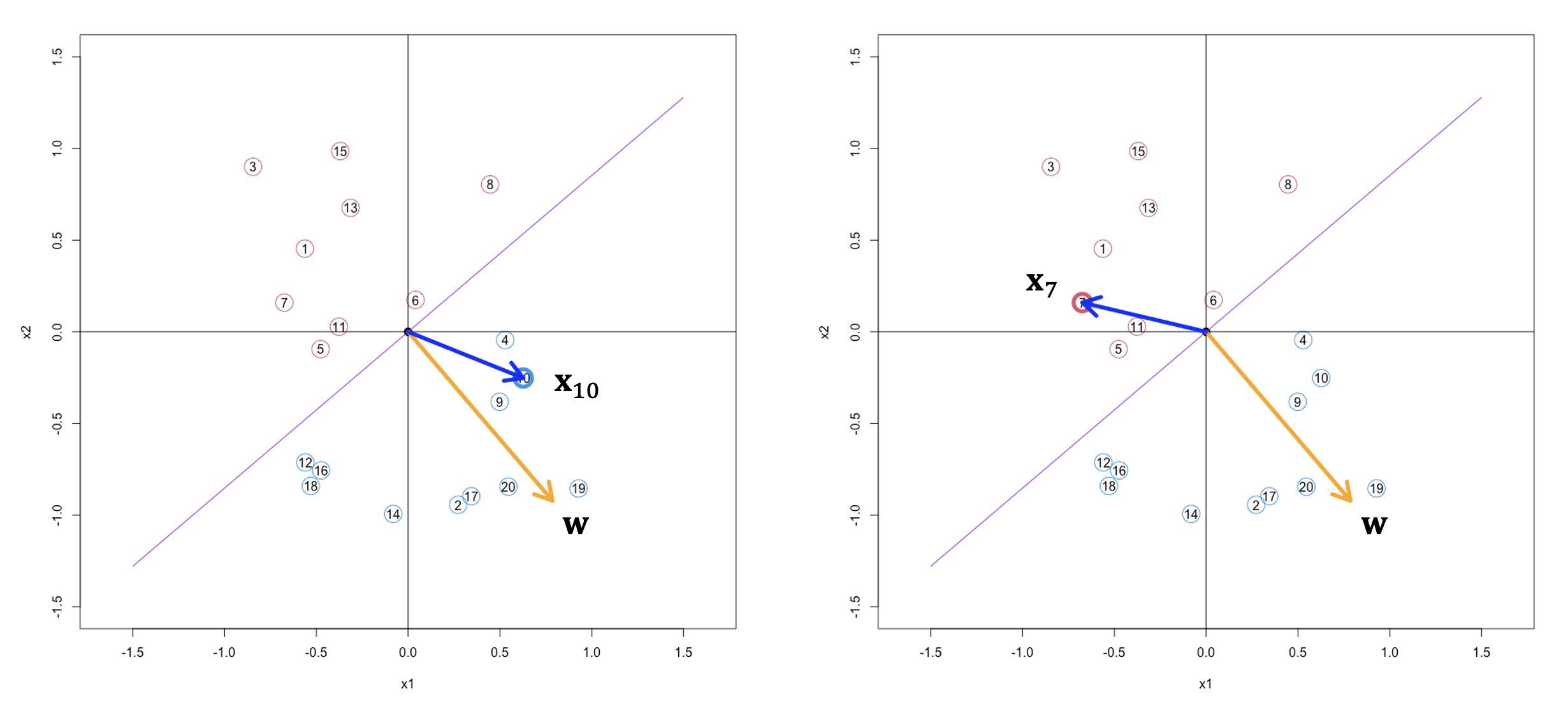
Based on this principle, let’s have look at a concrete example in the figure below.

