Basic Operators
In a space of vectors, we need to define some operations for studying the relations among vectors. In this section, we focus on two basic operations, i.e. scalar multiplication and addition, and their geometric meanings.
Scalar multiplication
For a vector \(\textbf{x} = \left( x_1, x_2, \dots, x_n\right)^{\top}\) and a scalar \(k\), \(k\cdot \textbf{x} = \left( kx_1, kx_2, \dots, kx_n\right)^{\top}\). In data science, scalar multiplication is very common, the simplest example would be we want to change the units of a variable. In the Swedish men’s height example, the units is M, if we want to change it to CM, then we actually calcluate
\[ 100\times(1.78, 1.85, 1.74, 1.82, 1.90, 1.88)^{\top} \] Scalar multiplication often appears in the form of weights as well. We will see more examples in the linear combination.
This operation can only change the magnitude (norm) of the vector, and you can verify the following equation \[ \|k\textbf{x}\| = k\|\textbf{x}\| \] From the geometric point of view, after doing this operation, the vector will be stretched.
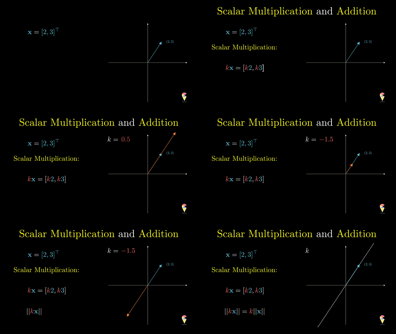
Also, \(k\textbf{x}\) represents a line in the direction of and crossing the original point.
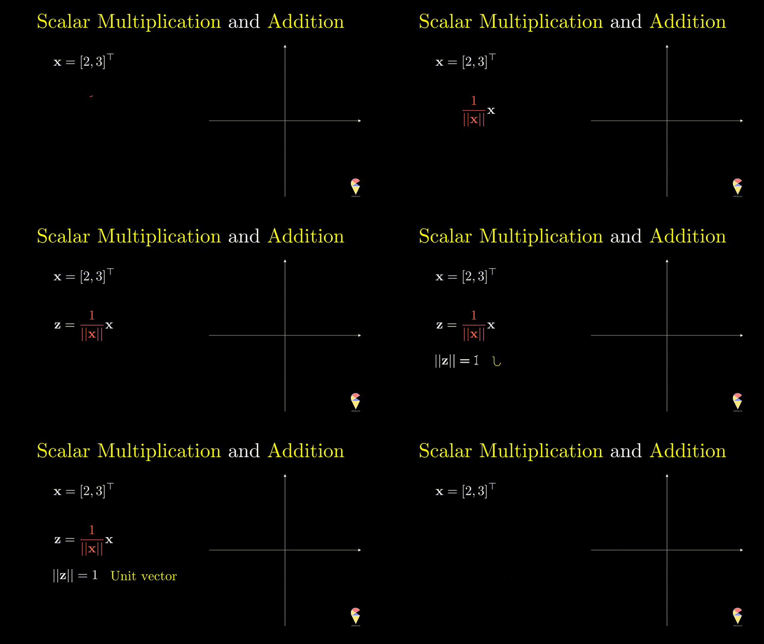
Given a vector \(\textbf{x}\) there is a special scalar multiplication if set \(k = \|\textbf{x}\|^{-1}\) since the length of the scaled vector is \(1\) and it is called the unit vector.
Addition
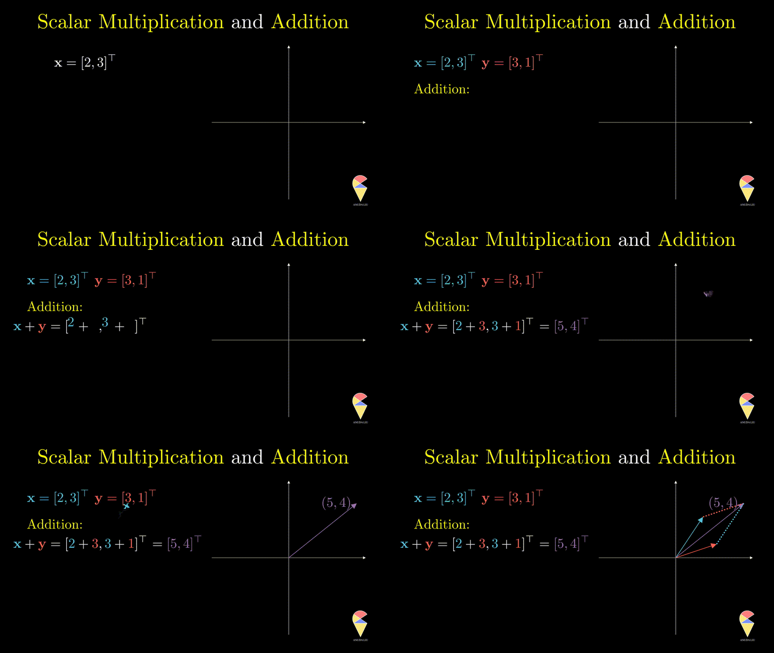
So far we have only considered single vectors and will consider the first operation on two vectors, addition. For vectors \(\textbf{x} = \left( x_1, x_2, \dots, x_n\right)^{\top}\) and \(\textbf{y} = \left( y_1, y_2, \dots, y_n\right)^{\top}\), \(\textbf{x} + \textbf{y} = \left( x_1 + y_1, x_2+y_2, \dots, x_n + y_n\right)^{\top}\)
From a geometric point of view, addition follows the so-called ‘parallelogram rule’:
- Two vectors complete a parallelogram, then the sum of the two vectors is the directed diagonal of the parallelogram.
The difference between two vectors can be viewed as the first vector adding the second vector which is rescaled by \(-1\)
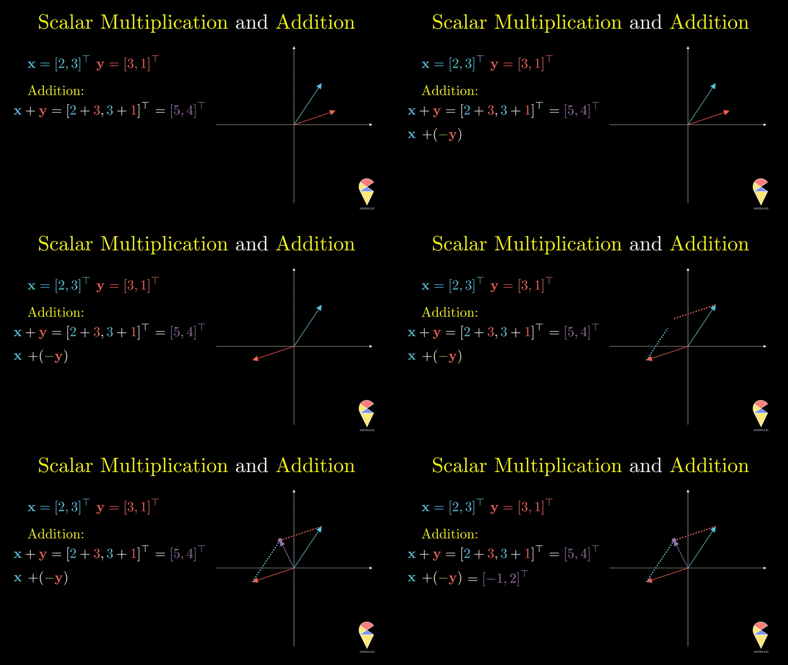
The last example essentially shows that the two vectors create the resulting purple vector through the two basic operations. ‘Create’ is the key word here, introducing the next concept, linear combination.
