Proceptron and Its Algorithm
Here, we introduce an old but interesting algorithm to train a classifier. The main purpose is help you getting real feelings about taring algorithm in machine learning and have a deeper understanding of linear classifiers.
Next, I’ll begin with a historical review of this algorithm and understanding the basic purpose of an machine learning algorithm. Then we use more algebra and geometry to show the intuitive idea behind of a linear classifier in general. In the end, the proceptron algorithm will be interpreted through algebra and geometry.
History
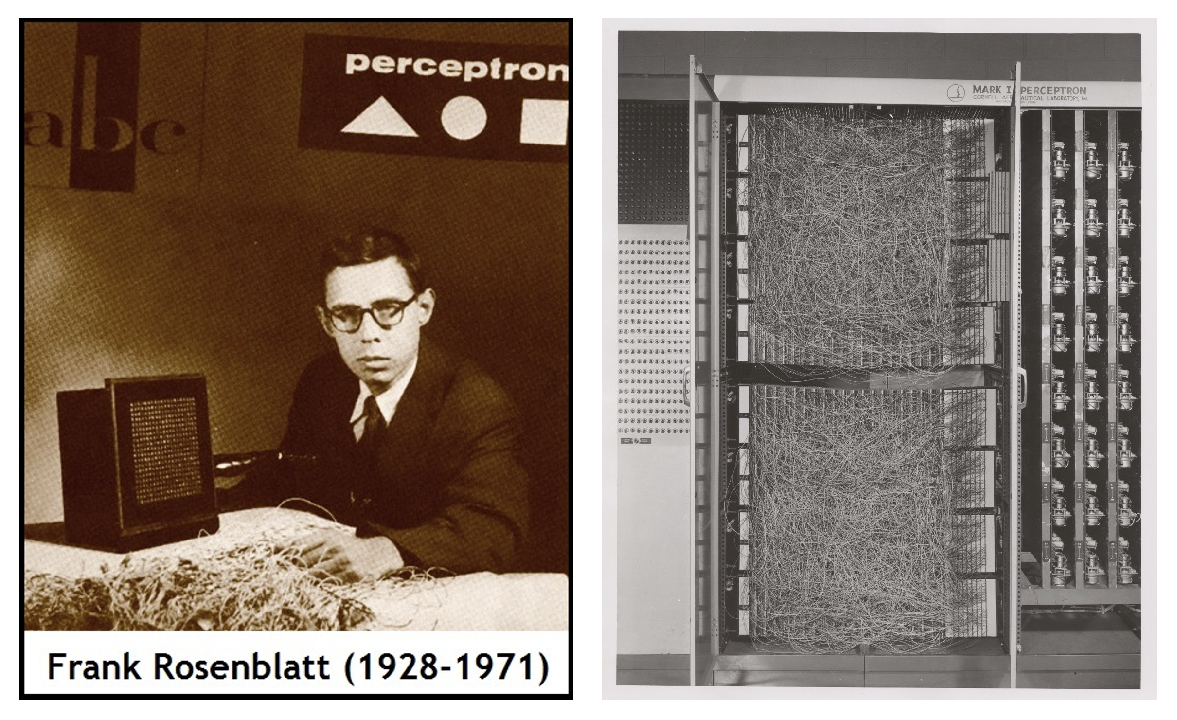
Proceptron classifier is viewed as the foundation and building block of artificial neural network. For a historical introduction, see the figures below.
Suppose we are solving a binary classification problem with \(p\) feature variables. As discussed before, it can be represented as
\[ \hat{y} = \text{Sign}( \textbf{w}^{\top} \textbf{x} + w_0 ) \]
where \(\textbf{w} = (w_1, w_2, \dots, w_p)^{\top}\), and \(\textbf{x} = (x_1, x_2, \dots, x_p)^{\top}\). Different from before, here we represent the weighted sum of \(p\) feature variables, \(w_1x_1+ \dots + w_px_p\), as the inner (dot) product of two vectors, i.e. \(\textbf{w} \cdot \textbf{x} = \textbf{w}^{\top} \textbf{x}\).
- Note: In order to understand proceptron algorithm, we need some basic knowledge about vector and its operations. If you are not familiar with it or need to refresh it, read about vector, operators, inner product before start reading the next.
The perceptron algorithm is about finding a set of reasonable weights. The key term here, “reasonable,” is easy to understand—it refers to a set of weights that can deliver good predictive performance. The core issue is how to find them.
- Brute-force idea: try all possible weight values and record the corresponding model performance, such as accuracy, and then choose the weights that yield the highest accuracy as the final model parameters.
However, this idea is clearly not ideal. Even if we only have two feature variables, this would still not be a simple task. A smarter approach is to do it this way: we start with an initial guess for the weight values, and then gradually approach the most reasonable weights through some iterative mechanism. This mechanism is called the perceptron algorithm. Next, let’s dive into learning this magical mechanism—the perceptron algorithm.
Next, the logic goes like this:
- Further explore the geometric properties of linear classifiers
- Use geometry to understand how this algorithm works.
Geometry of Linear Classifiers
Note: From now, we will temporarily ignore the bias term, \(w_0\), or assume it as \(0\). It will not influence our final conclusion. No worries. So, the basic classifier is represented as \(y = \text{Sign}(\textbf{w}^{\top}\textbf{x})\)
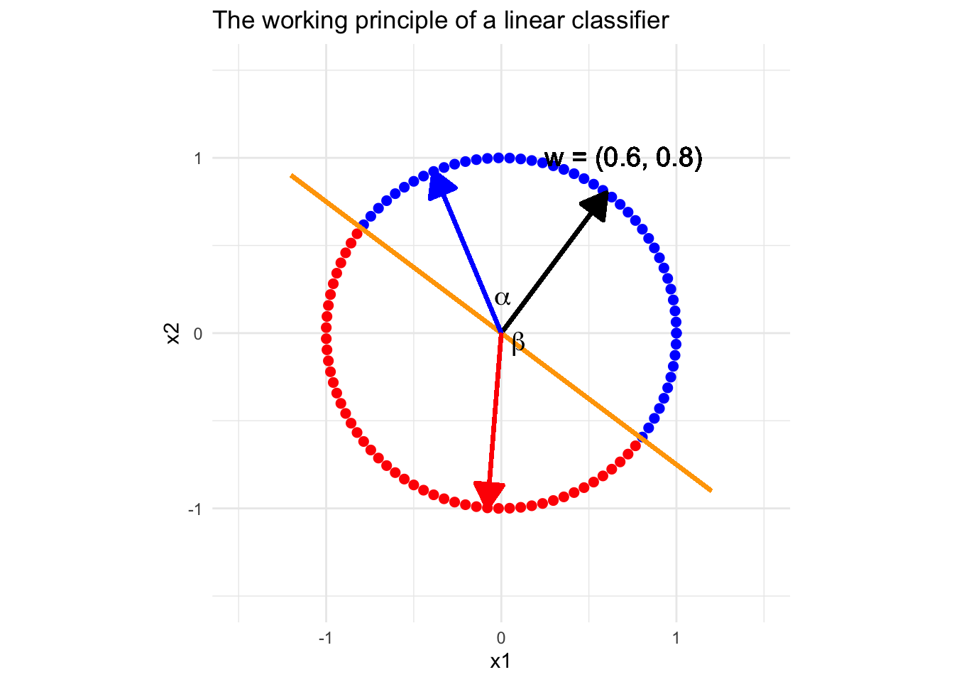
Previously, we explored the geometric understanding of linear classifiers, which is that the classifier determines a linear decision boundary. Next, let’s understand a linear classifier from another view of geometry. Suppose we have a classifier with two feature variables, \(x_1\) and \(x_2\), and the “reasonable” weight vector is \(\textbf{w} = (0.6, 0.8)^{\top}\). Look at the conceptual plot below.
It is easy to see that all the vectors (points) in blue form a sharp angle with the weights vector (black). By the property of inner product, (read about inner product) for any point \(\textcolor{blue}{\textbf{x}} = (\textcolor{blue}{x_1},\textcolor{blue}{x_2})^{\top}\) standing on the direction pointed by the blue arrow, \(\textbf{w}^{\top}\textcolor{blue}{\textbf{x}} \propto \cos(\alpha) > 0\), i.e. all the cases on this direction will be classify as positive. On the contrary, all the vectors (points) in blue form a obtuse angle with the weights vector, and then \(\textbf{w}^{\top}\textcolor{red}{\textbf{x}} \propto \cos(\beta) < 0\), i.e. all the points standing on the direction pointed by a red vector will be classified as negative. With this observation, we can easily understand how does a “reasonable” linear classifier work.
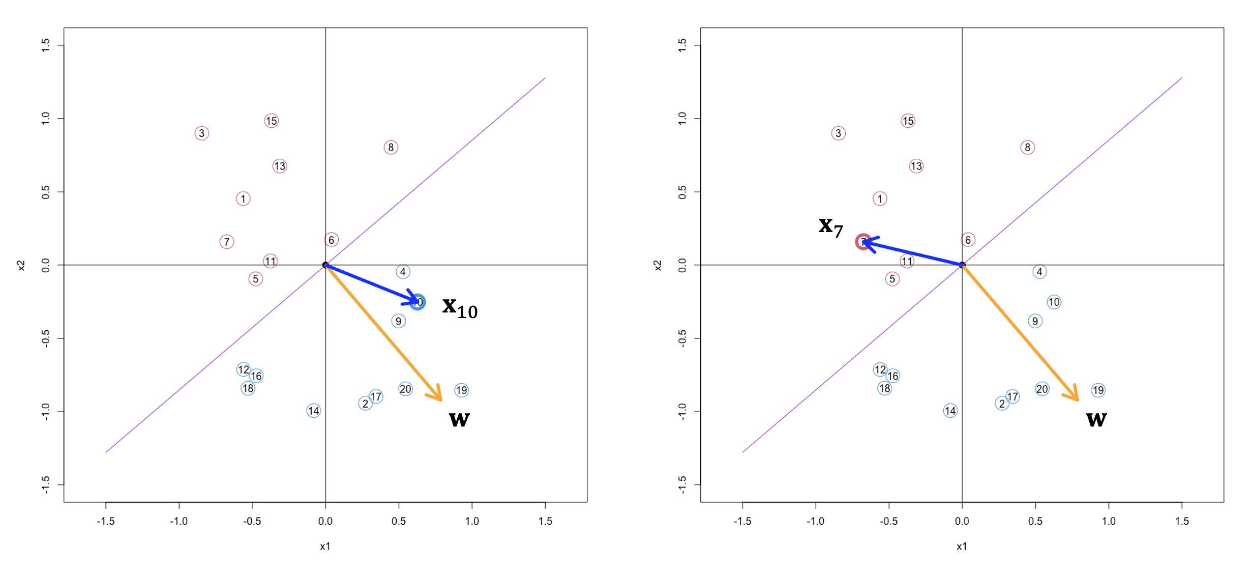
Based on this principle, let’s have look at a concrete example in the figure below.
Proceptron Algorithm
With the discussion above, at least for me, the weights vector of a perceptron classifier is like a sword of judgment, wielded to evaluate all cases. So, I just name proceptron algorithm as finding sword of judgment algorithm. You may remember the brute force idea, so the next question is whether we have a clever way to quickly find the sword of judgment instead of trying all possibilities.
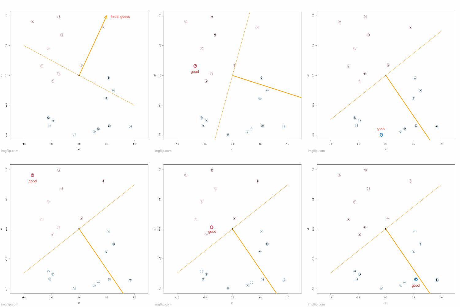
Before we begin to understand how this algorithm works, we must first reach a consensus that no matter how we look for it, we must have a starting point, and this starting point is preferably random. If you agree with me, let’s randomly pick up one initial guess of the sword (weights vector) in the following conceptual example.

This initial guess is not too bad since it only made one mistake, see the 2nd column of the image. This case is a positive case but wrongly predicted as negative. So, we need to correct this weights vector such that the corresponding decision boundary will be rotated clockwise slightly. From the 3rd column of the image we can see that, this aim can be achieved by updating the weights vector as \[ \textcolor{red}{\textbf{w}}^{\text{new}} = \textcolor{green}{\textbf{w}}^{\text{old}} + \textcolor{blue}{\textbf{x}} \]
By the Parallelogram Law (read about vector addition), the old weights vector will be rotated clockwise, thereafter the decision boundary is corrected properly.
Suppose the mistake by the initial guess of sword (\(\textbf{w}\)) happened for a negative case, see figure below. In this case, we need to update the weights vector as
\[ \textcolor{red}{\textbf{w}}^{\text{new}} = \textcolor{green}{\textbf{w}}^{\text{old}} - \textcolor{red}{\textbf{x}} \]
such that the decision boundary will be anticlockwise slightly.

Notice that the target variable \(y = -1\) or \(+1\), therefore we can integrate the two updating rule as one:
\[ \textcolor{red}{\textbf{w}}^{\text{new}} = \textcolor{green}{\textbf{w}}^{\text{old}} + y \textbf{x} \]
Now, we have actually found a clever way to search for the sword of judgment. Basically, we can do this. First, number all cases, and then randomly pick an initial guess for \(\textbf{w}\). After these are prepared, we start to use this sword to test cases in the order of numbers. If we find a wrong judgment, such as number 3, then we correct this sword according to the updating formula above. After the correction, continue to judge in order, that is, start judging from number 4, and continue to correct the error. Repeat this process, and when we find a real sword that can correctly judge all cases, we stop the search process. This is the so called Proceptron Algorithm:
Proceptron Algorithm:
Inputs: y nx1 vector taking vaules -1 or 1, X nxp matrix
Initialization: weight vector w randomly initialized

While(All cases are correctly classified){
  for(i in 1:n){
    if(case i is misclassified){
      w = w + y[i]X[i, ]
    }
  }
}
Below, you can see an animation presenting the Proceptron Algorithm in action.
Remarks:
- This algorithm works, that is, as long as we follow this algorithm, no matter where we start, we can always find the sword of judgment.
- However, as you may have realized, this algorithm has a prerequisite, that is, our training samples are linearly separable. In other words, we can find a straight line (2D case) to split the sample space, all positive and negative examples stand on each side, or we will not make any mistakes in the training samples.
- In addition, you may also find that the “reasonable” \(\textbf{w}\) obtained by this algorithm is not unique, that is, there exist many swords of judgment, and which one we finally get depends on our initial guess.
