3.5 Continuous Random Variables
Next, we will consider a more challenging concept, continuous random variable. As you may notice, all the random events that we are considering can be represented by categorical outcomes. For example, flipping a coin has two outcomes, throwing a dice has 6 outcomes, and so on. For this kind of random event, it is sufficient to consider random variables only taking integer values. Thus we refer to the random variables discussed as discrete random variables. In practice, however, there are many other random events whose outcomes are not categorical but continuous values, for example, the temperature, the height of adult males, and so on. Therefore we need another type of random variable, a continuous variable.
3.5.1 Continuous distribution
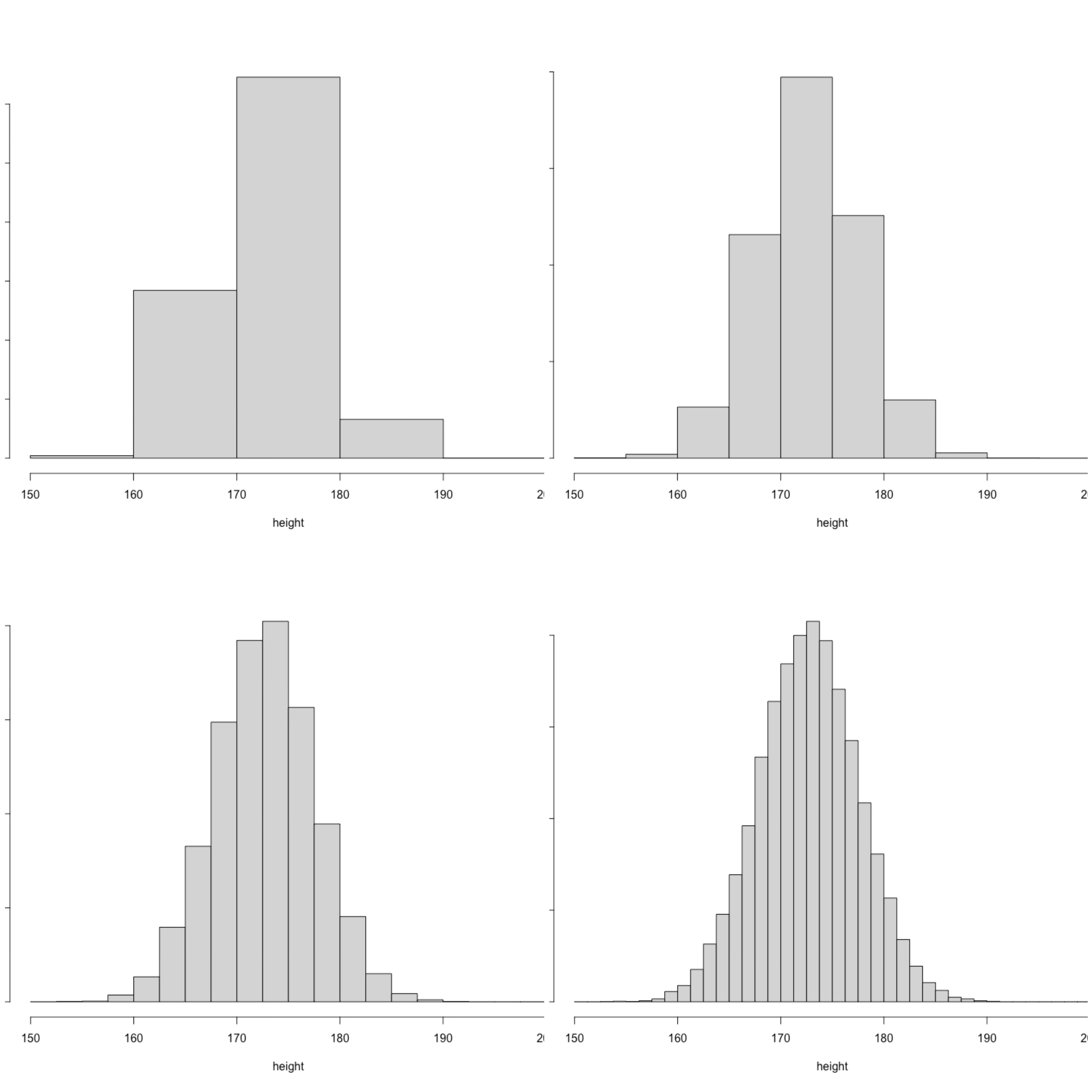
Continuous random variables are not difficult to understand, they are nothing more than random variables that take real numbers, but the problem is how to describe their distribution. Again, let us abstract mathematical concepts from reality. Let’s consider such a background problem, assuming that I have height data for all boys in middle school in Sweden. Height is obviously not a categorical variable, but we can still use grouping to describe the distribution of height from a discrete perspective. Specifically, we can evenly divide the possible range of height into several groups, and then calculate the percentage of the number of people in each group to the total number of people. Yes, if you are familiar with basic statistics, you can tell that this is a histogram at a glance.

Such an approach has obvious flaws. For example, on the left-top of the plot, it is difficult for us to distinguish the probability of height being less than 175 and greater than 170 because these two values are combined into one group. How to do it? Very simple, we can split each large group into two small groups, of course, you also need to include more boys into the data set and then calculate the frequency of each group to represent the distribution of height, for example, on the right-top of the plot. If we still cannot distinguish the above probability, we can continue to split each group into two groups. Doing this we can see that the histogram is more detailed. If we have a sufficient large data set, we can continue to subdivide the height group and know the probability that we can distinguish the above two events. Suppose we put “all” the boys in middle school into this histogram, and each group can be subdivided infinitely. We can imagine that the upper edge of the histogram will be a smooth curve. We call this smooth curve the probability density function (p.d.f) and denote it as \(f(x)\). A valid p.d.f has to inherit two conditions from the p.m.f of a discrete random. First, the density value must be positive, \(f(x) > 0\), and the integral on the whole domain should be 1, \(\int_{-\infty}^{\infty} f(x) dx = 1\). With this function, we can calculate the probability of many events, as well as the expectation and variance. \[ \Pr(X<b) = \int_{-\infty}^bf(x)dx \] \[ \text{E}(X) = \int_{-\infty}^{\infty} xf(x) dx \]
One can compare the formula above with the expected value of a discrete random variable, \(\text{E}(X) = \sum_k k\Pr(x=k)\). You can see similar patterns, they all are the “sum” of all possible values times the corresponding probability or density values. Keep in mind that the integral symbol is an elongated S which indicates “sum”.
So far, we have only specified the basic conditions for a function to be a p.d.f , but the exact form of this function depends on the continuous distribution it represents. Next, we will learn about one of the most common continuous distributions: the Normal distribution.
3.5.2 Normal (Gaussian) distribution
A continuous random variable is Normally distributed, \(X \sim \mathcal{N}(\mu, \sigma^2)\), if its density function is
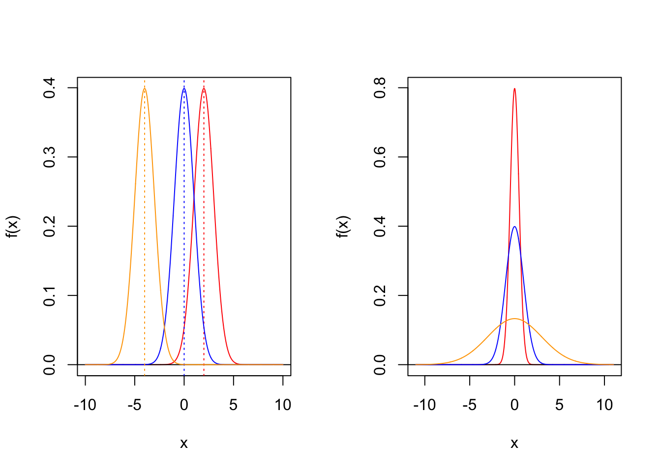
\[ f(x) = \frac{1}{\sigma \sqrt{2 \pi} } e^{- \frac{1}{2} \left( \frac{x-\mu}{\sigma}\right)^2 } \] The normal distribution is determined by two parameters, location parameter \(\mu\) and shape parameter \(\sigma^2\). Density functions of normal distribution with different parameters are displayed in the following picture.
Now, I have two questions to you.
We have studied both discrete random variable and continuous random variable, their distribution of possible values can be presented by p.m.f and p.d.f respectively. The value of a p.m.f is just the probability when the random variable taking this value. However, what is the meaning of the value of a p.d.f?
What is the essence of the Normal distribution? In simpler terms, how would you introduce the concept of the Normal distribution to a middle school student?
Think about them and we will come back to them later on.
