3.4 Two Dependent Random Variables
3.4.1 Sum rule and product rule
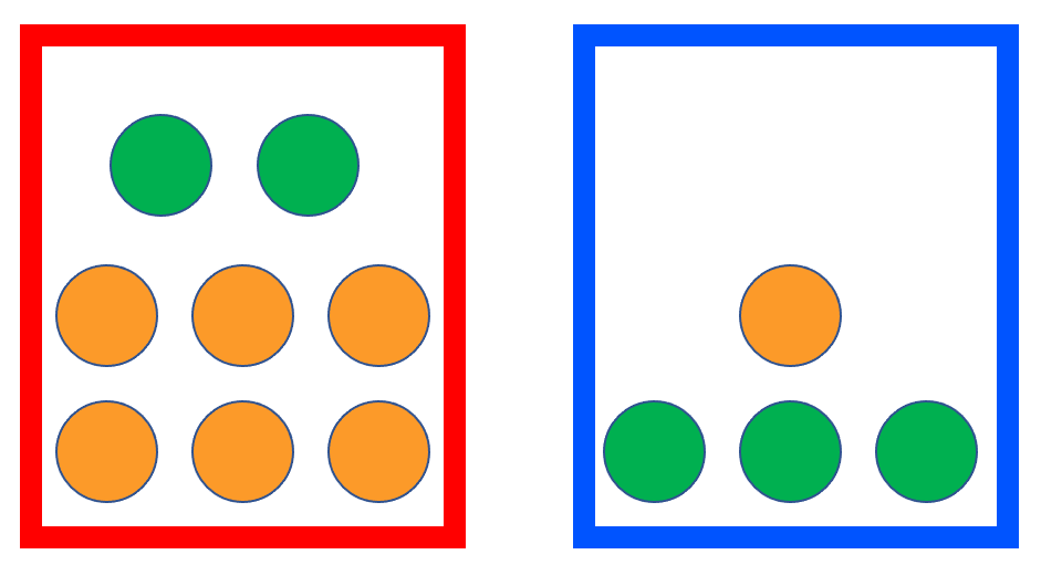
Let’s think about a question like this. The basic conditions are presented in the following picture. Suppose we want to randomly pick a box and then randomly take out a fruit from it, then what is the probability that the fruit taken out is an apple? We can randomly pick the box by throwing a dice. If we get a number less than 5 then we choose the red box, or we choose the blue box.

This example is a bit more complicated than the previous because there are two randomized actions involved here. The result of this action involves a combination of the color of the box and the type of fruits. Let’s start by considering the probability that the red box is drawn while an apple is picked up. Again, we can use the previous formula to calculate this probability. There are six numbers corresponding to the dice, and the number of fruits inside the red box is 8, so all the possibilities are \(6 \times 8\). But there are only numbers 1 through 4 and two apples, so there are only \(4 \times 2\) possibilities that qualify. So the probability is \[ \frac{4\times2}{6\times8} = \frac{4}{6} \times \frac{2}{8} = \frac{1}{6} \] It is easy to see that \(4/6\) is the probability of getting a number less than \(5\), i.e. the red box is selected. But what is the meaning of the second part, \(2/8\)? Since \(8\) is the number of fruits and \(2\) is the number of apples in the red box, it can be understood as the probability of getting an apple when the red box was selected. We refer to this probability as conditional probability and present it as \(\Pr(\text{Apple} | \text{Red}) = 2/8\). This discussion can be summarized as \[ \Pr ( \text{Red AND Apple} ) = \Pr( \text{Apple} | \text{Red} ) \Pr ( \text{Red} ) \] We can also easily get the probability of getting an apple under the other possibility, i.e. \[ \Pr(\text{Blue AND Apple}) = \Pr(\text{Apple} | \text{Blue} ) \Pr( \text{Blue} ) = \frac{3}{4} \times \frac{2}{6} = \frac{1}{4} \] “AND” corresponds to the “product rule”. \[ \Pr(E_1 \text{ AND } E_2) = \Pr(E_1 | E_2)\Pr(E_2) = \Pr(E_2 | E_1)\Pr(E_1) \] Going back to our original question, what is the probability of getting an apple? This random event can be labeled as “Red AND Apple OR Blue AND Apple”. Here, we have the second rule, i.e. “sum rule”, when considering the “OR” operator between two events that don’t happen simultaneously. \[ \Pr(E_1 \text{ OR } E_2) = \Pr(E_1) + \Pr(E_2) \]
Based on the sum rule, the probability of getting an apple is calculated as \[ \Pr( \text{Apple} ) = \Pr( \text{Red AND Apple} ) + \Pr( \text{Blue AND Apple} ) = \frac{5}{12} \]
Remark: we can compare it with the sum-product rule in permutation and combinations. When there are different types of solutions for one thing, the total number of possible solutions is the sum of the number of possible solutions for each type. When there are different steps in doing one thing, the total number of solutions is the product of the number of possible solutions in each step.
3.4.2 Joint distribution and marginal distribution
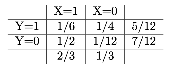
Similarly, you can verify the probabilities when orange is considered. If we use random variables to present the events, for example, the random variable \(X\) presents the box selected, \(1\) indicates red, and \(0\) indicates blue; the random variable \(Y\) presents the fruit drew, then the following table is called the joint distribution of two random variables.

The last column is called the marginal distribution of random variable \(Y\), and the last row is the marginal distribution of random variable \(X\).
3.4.3 Posterior and Prior Probabilities
With the example above, the last interesting question is “What is the probability we chose the blue box if we get an orange?” First of all, it is a conditional probability, \(\Pr(X = 0 | Y = 0)\). According to the product rule, we know that this conditional probability is the ratio between \(\Pr(X=0 \text{ and } Y=0)\) and \(\Pr(Y=0)\). The first second has been calculated before and that is \(7/12\). Well, the first can be calculated by product rule again, i.e. \(\Pr( Y = 0 | X = 0 ) \Pr(X=0)\). Summarize, \[ \Pr(X = 0 | Y = 0) = \frac{\Pr( Y = 0 | X = 0 ) \Pr(X=0)}{\Pr(Y=0)} \]
\(\Pr(X=0|Y=0)\) is different from the conditional probability in the first question \(\Pr(Y=0|X=0)\). This probability is referred to as the posterior probability in the sense that we use the observation in the second step to update the probability of the first step. Correspondingly, the probability of drawing a blue box at the first step is called prior probability. The formula above is well known as Bayes formula.
3.4.4 Statistically independent
From the joint distribution, the probability of drawing an apple \(\Pr(Y = 1)\) is \(5/12\). It is different from the probability of drawing an apple under the condition that the red box was selected, \(\Pr(Y=1 | X = 1) = 2/8\). This fact implies that the value of random variable \(Y\) depends on the value of \(X\), or random variable \(X\) and \(Y\) are dependent. If we add 1 apple and 11 oranges to the blue box, then \(\Pr(Y=1) = \Pr(Y=1 | X = 1)\). In this case, the value of random variable \(Y\) doesn’t depend on the value of \(X\), i.e. they are independent.
3.4.5 Covariance and Correlation
For two random variables \(X\) and \(Y\), we can use covariance to quantify the degree of association between two random variables. The covariance is defined as \[ \text{Cov}(X, Y) = \text{E}(X-\text{E}(X))(Y-\text{E}(Y)) \] The mean and variance of a weighted sum (linear combination) of two random variables are \[ \text{E}(aX+bY) = a\text{E}(X) + b\text{E}(Y) \] and \[ \text{Var}(aX+bY) = a^2\text{Var}(X) + 2ab\text{Cov}(X,Y) + b^2\text{Var}(Y) \] respectively.
Another characteristic value that quantifies the correlation between two variables is correlation. It is simply normalized covariance, i.e.
\[ \rho_{x,y} = \frac{\text{Cov}(X, Y)}{\sqrt{\text{Var}(X)} \cdot \sqrt{\text{Var}(Y)}} \] When the two variable uncorrelated, \(\text{Cov}(X, Y) = 0\), therefore \(\rho_{x,y} = 0\). Another two extreme cases are \(X = Y\), i.e. two random variables are the same, and \(X = -Y\). In these cases, \(\text{Cov}(X, \pm Y) = \pm \text{Cov}(X, X) = \pm \text{Var}(X)\), therefore, \(\rho_{x,y} = \pm 1\). Thus, different from covariance, the correlation is a number between \([-1, 1]\) due to the normalization. So, it is more comparable than covariance and people often use it to quantify the association between variables.
