dnorm(179,179,5.5) [1] 0.07253496dnorm(230,179,5.5)[1] 1.546941e-20Likelihood analysis is an important concept in the modern statistics. A good understanding of likelihood can help you improve your knowledge in statistics. By understanding the relationship between likelihood and probability, you can build a bridge in statistical or data and probability modeling, allowing you to use models with greater confidence.
We have build up all the basic concepts of probability. In simple terms, probability is a mathematical model used to quantify the possibility of an event. The discussion of the possibility of this event is limited to the realm of rationality. For example, we can use probability to discuss the following questions.
“Imagine you are standing in the square in the city center of Umeå, close your eyes for 30 seconds, then open your eyes and catch the first man you see. How likely is his height above 180 cm?”
Let’s have a look at another scenario,
“You went to downtown last weekend. You stood in the square and closed your eyes, then after 30 seconds you opened your eyes and grabbed the man you saw first and measured his height. His height is 230 and you think it is unbelievable.”
In this case, we have a real observation of a random variable and want to evaluate the possibility of this observation. In this case, a proper word is likelihood value. I hope from the two examples above, you can see the difference between the two synonyms for “possibility.” In one word, likelihood value is the evaluation of the possibility to one observed valued, but probability evaluate the possibility of an event (somehow have not happened). Now, we can answer the first question above, what is the meaning of the value of a p.d.f? It present the likelihood of a real observation. For example, we may assume the height of adult men in Sweden is Normally distributed with mean 170 and SD 5.5 (I got these statistics from SCB, Statistiska centralbyrån), then the likelihood values of observing a man who is 179 and a men who is 230 are
So, it is almost impossible to see a men who is 230 in the center of Umeå city.
Remark 1: Unlike probability, likelihood is not standardized and is not a decimal between 0 and 1. When the standard deviation is very small, the likelihood value near the mean can be quite large. For example,
Remark 2 (HBG2K) : When people use the likelihood value, they often take the logarithm of it. One reason is that, even when the likelihood value is very small, we can still have a meaningful number for calculations. Another reason is that the distributions we commonly use, like the normal distribution, belong to the exponential family, so taking the logarithm transforms a nonlinear function into a linear one. For example,
Next, we summarize the facts about discrete random variable and continuous random variable in the following table.

You surely remember the previous question: what does the p.d.f of the normal distribution represent?
\[ f(x) = \frac{1}{\sigma \sqrt{2 \pi} } e^{- \frac{1}{2} \left( \frac{x-\mu}{\sigma}\right)^2 } \]
Or, to put it another way, just as the binary distribution aims to describe random events like coin tossing, what kind of random phenomenon is the normal distribution trying to describe?
Let’s start with en elementary understanding.
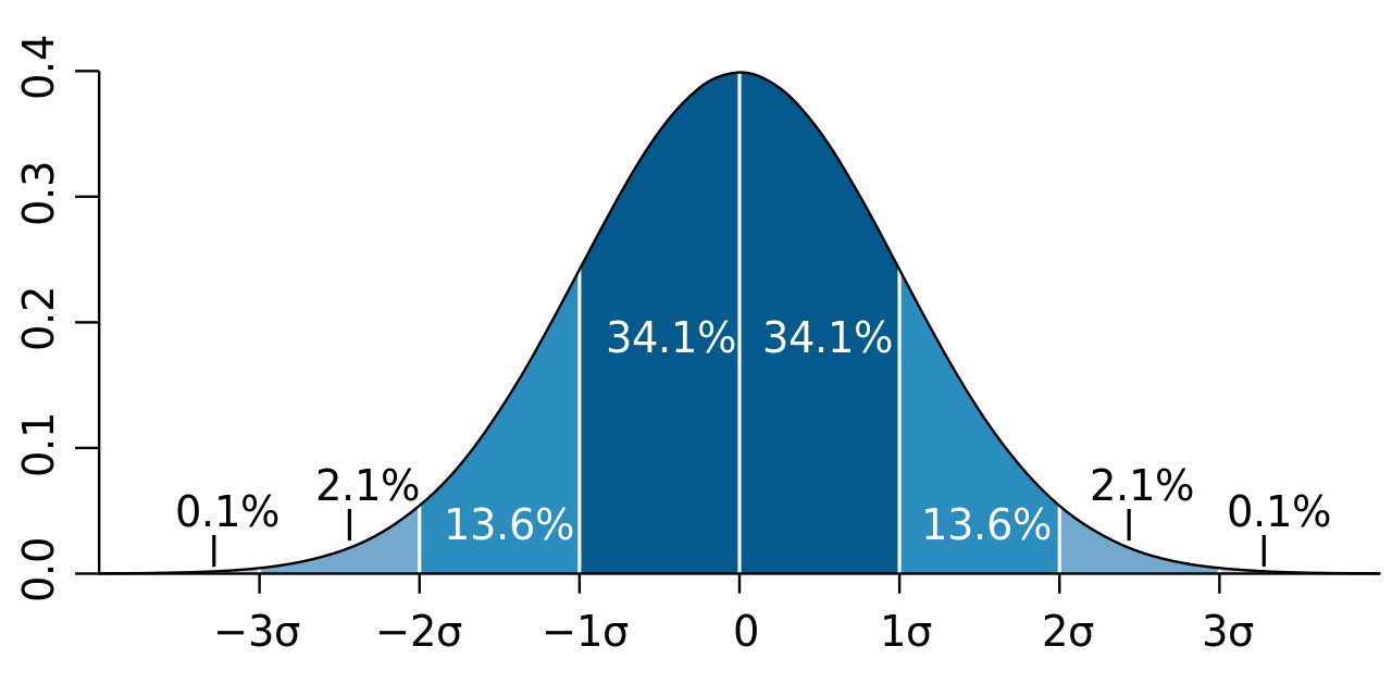
The normal distribution describes a bell-shaped, symmetric distribution of random phenomena, such as human IQ. Most people’s IQs are close to the mean, a smaller portion have higher or lower IQs, and only a very few have extremely high or low IQs. This forms a bell-shaped, symmetric distribution.
We can use more precise statistical terminology, such as confidence intervals, to describe this bell-shaped symmetric distribution of random phenomena. The normal distribution describes a random phenomenon where 68% of the probability is covered by the confidence interval of one SD around the mean, while the confidence interval of two SDs can cover 95% of the probability, and the confidence interval of three SDs can cover nearly all possibilities, as shown in the figure below.”
If you answer the question in such ways, then congratulations. You have rather good learning outputs from the previous basic statistics course. Next, let me introduce to you a deeper understanding based on the concept of likelihood. Let’s review the p.d.f of the normal distribution. Let’s watch an animation first.

Notice that \(\left(\frac{x-u}{\sigma}\right)^2\) is the normalized distance between an observation \(x\) and the center point \(\mu\). As mentioned before, the value of density function is the likelihood value of one observation, so the p.d.f is presenting the relationship between a specific observation \(x\) and its likelihood value. Then Normal distribution is describing such kind of random phenomenon:
The likelihood of an observation \(x_0\) is inversely proportion to the normalized distance between observed value \(x_0\) and the mean value \(\mu\).
More precisely, when the observed value is far from the center point, the likelihood of observing it will decrease rapidly, and this decrease is exponential, as displayed below.

In summary, the normal distribution essentially describes the relationship between the distance of observed values from the center point and likelihood within a class of random phenomena. It connects the geometric concept of distance with the statistical concept of likelihood.
With the likelihood idea, we can easily extend the normal distribution to a multidimensional case. In this note, I will just list several points help you to understand the main idea.
What is multidimensional case? For example, we may assume the height of Swedish adult men is normally distributed and denote as \(X_1 \sim \mathcal{N}(\mu_1, \sigma_1^2)\). We also know that another important physical indicator is weight, which can also be assumed to follow a normal distribution, denoted as \(X_2 \sim \mathcal{N}(\mu_2, \sigma_2^2)\). If, for each Swedish adult man, we simultaneously consider height and weight as descriptive features rather than just one or the other, then we enter a multidimensional scenario. So, what changes do we need to make in a multidimensional scenario? With the height-weight example,
We need two values to determine the location of the center point of the distribution, or we need a mean vector \((\mu_1, \mu_2)^{\top}\).
In the one dim case, we use variance/SD to control the shape of distribution. Naturally, we also need to consider the two variance simultaneously. However, this isn’t sufficient. We also need to take the association between the two variables, i.e. covariance, into account, as it is also an important factor in determine the overall shape. So, we need a covariance matrix to contain all the shape information, for example, in 2D case, \[ \left( \begin{matrix} \text{Var}(\text{Height}) & \text{Cov}(\text{Height}, \text{Weight}) \\ \text{Cov}(\text{Height}, \text{Weight}) & \text{Var}(\text{Weight}) \end{matrix} \right) \] Usually, a covariance matrix is denoted by \(\boldsymbol{\Sigma}\) which is a \(p \times p\) symmetric matrix (also need to be positive definite), \(p\) is the number of variables. In 2D case, the covariance matrix is usually presented as \[ \boldsymbol{\Sigma}= \left( \begin{matrix} \sigma_1^2 &\sigma_{12}\\ \sigma_{12} & \sigma_2^2 \end{matrix} \right) \] Given the definition of correlation, it is also can be represented as \[ \boldsymbol{\Sigma}= \left( \begin{matrix} \sigma_1^2 & \rho \sigma_1\sigma_2\\ \rho \sigma_1\sigma_2 & \sigma_2^2 \end{matrix} \right) \] where \(\rho\) is the correlation between \(X_1\) and \(X_2\)
We explained what is the essence of Normal distributions, that is likelihood value of an observation is inversely proportional to the normalized distance between the observation and mean value. Multivariate normal distribution should inherent this idea for sure. But the question is what is the normalized distance in 2D? Well, it is not such straightforward, I will explain it in another notes. (ToDo4Sia) We can just understand it as some normalized Euclidean distance in 2D. Thus, normal distributions, regardless of their dimensional, share a common pattern in their p.d.f , i.e. \[ f(\textbf{x}) \propto \exp ( - d_M(\textbf{x}, \boldsymbol{\mu}) ) \] where \(\textbf{x} = (x_1, x_2)^{\top}\), \(\boldsymbol{\mu} = (\mu_1, \mu_2)^{\top}\) and \(d_M(\cdot, \cdot )\) is the normalized distance between two input points. From the LHS of the formula, in in the 2D setting, the likelihood value of each observation (man) is determined by two inputs. From the RHS of the formula, the likelihood value is determined by the normalized distance \(d_M\), i.e. closer to the center point, higher possibility to observe.
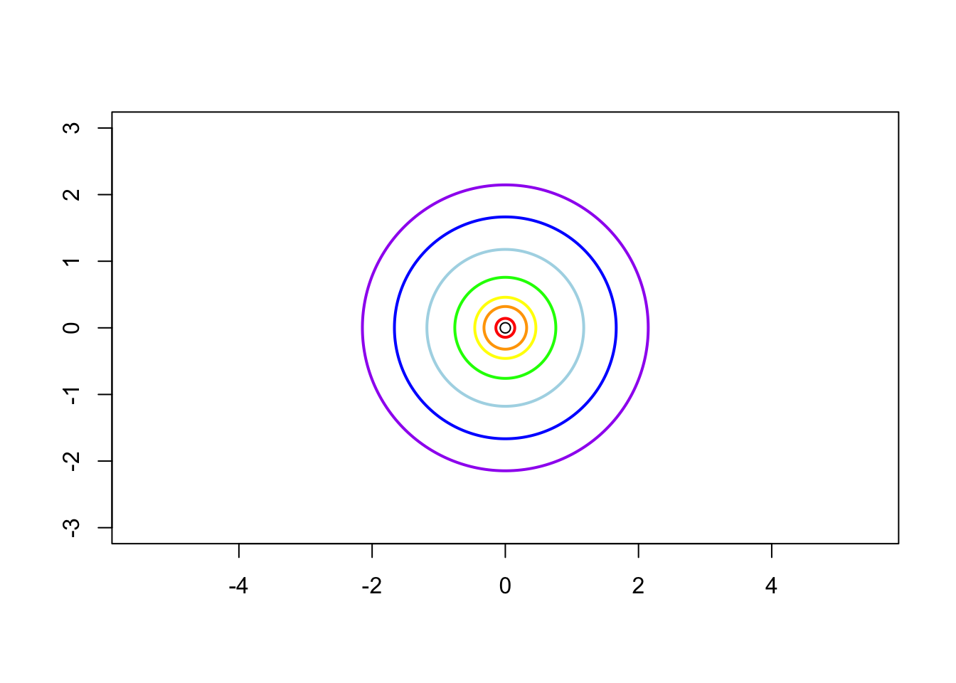
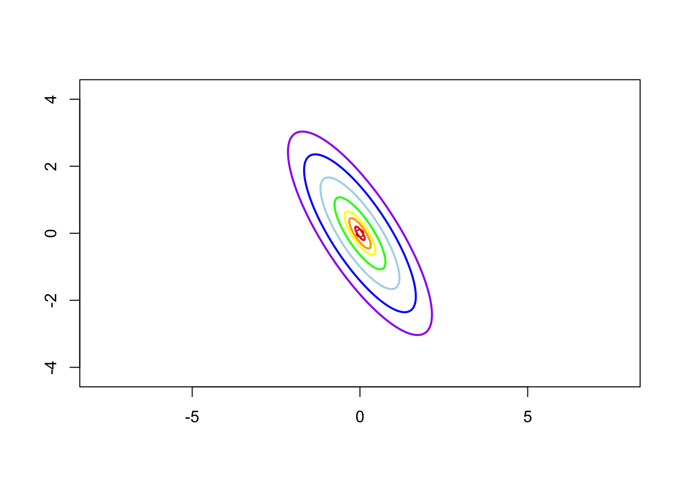
Next, I show you some examples to demonstrate the arguments above.
Case 1: \(\sigma_1^2 = \sigma_2^2 = 1\) and \(\rho = 0\), i.e. the contrivance matrix is \[ \boldsymbol{\Sigma} = \left( \begin{matrix} 1 & 0 \\ 0 & 1 \end{matrix} \right) \]
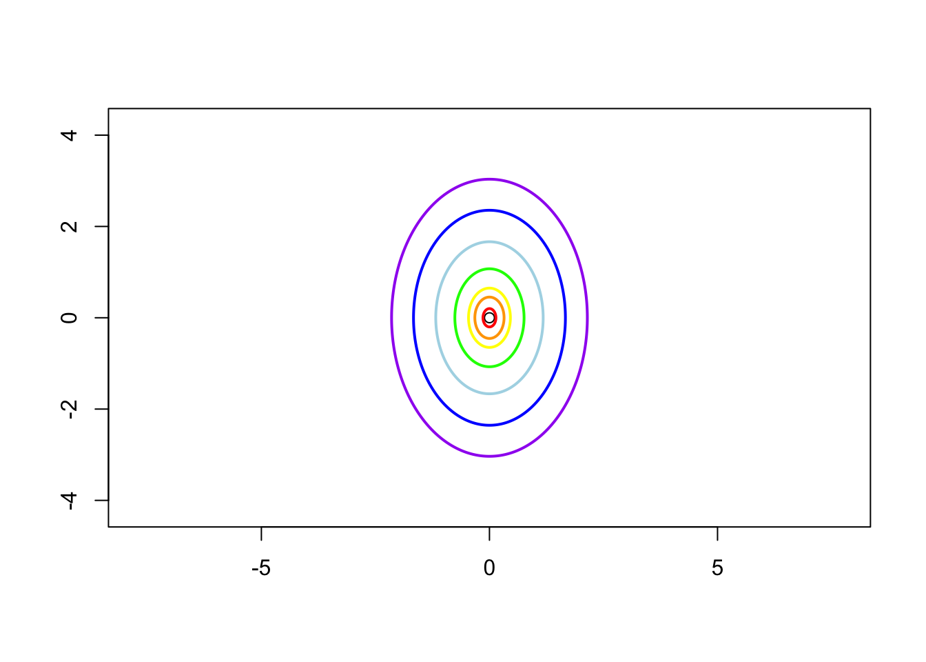
Case 2: \(\sigma_1^2 = 1\), \(\sigma_2^2 = 2\) and \(\rho = 0\) i.e. the contrivance matrix is \[ \boldsymbol{\Sigma} = \left( \begin{matrix} 1 & 0 \\ 0 & 2 \end{matrix} \right) \]
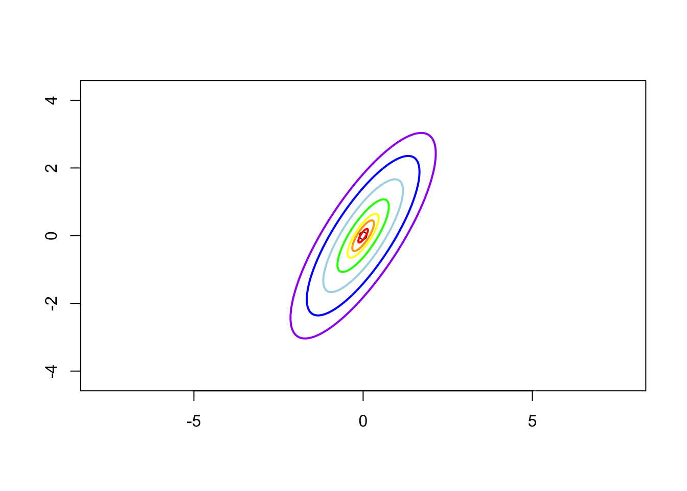
Case 3: \(\sigma_1 = 1\), \(\sigma_2 = 2\) and \(\rho = 0.8\), i.e. the contrivance matrix is \[ \boldsymbol{\Sigma} = \left( \begin{matrix} 1 & 1.13 \\ 1.13 & 2 \end{matrix} \right) \]
Case 4: \(\sigma_1 = 1\), \(\sigma_2 = 2\) and \(\rho = -0.8\), i.e. the contrivance matrix is \[ \boldsymbol{\Sigma} = \left( \begin{matrix} 1 & -1.13 \\ -1.13 & 2 \end{matrix} \right) \]
There are more stories about Normal (Gaussian) distribution. I will write a note about it. Please keep an eye on my space. ToDo4Sia: write a note telling the story of Gaussian distribution.
