In the previous section, we discussed what PCA is and the optimization problem it involves. This optimization problem is actually quite easy to solve because it is equivalent to an eigenvalue decomposition problem. Here, we will skip the mathematical details and directly present the algorithm, explaining how to obtain PC weights and use them to compute the new data matrix. Finally, we will demonstrate this with a small example.
Algorithm: Principal Components Analysis
Inputs:
\(\textbf{X}\), \(n\times p\) matrix, containing all \(p\) feature variables.
Steps:
Calculate the covariance matrix, \(S_{\textbf{X}}\)
Perform eigenvalue decomposition on the covariance matrix, \(S_{\textbf{X}} = \textbf{W} \boldsymbol{\Lambda} \textbf{W}^{\top}\). \(\mathbf{W}\) is a \(p \times p\) matrix, where each column, \(\textbf{w}_j\), is an eigenvector, and we call it weights matrix. \(\boldsymbol{\Lambda}\) is a diagonal matrix, where each diagonal element \(\lambda_j\) is the eigenvalue corresponding to its eigenvector \(\textbf{w}_j\).
Calculate the new data matrix: \(\mathbf{Z} = \mathbf{XW}\)
Output: The new data matrix, \(\mathbf{Z}\), the weights matrix, \(\mathbf{W}\), and the matrix of eigenvalues, \(\boldsymbol{\Lambda}\).
First, it is not difficult to guess that the PC weights we are looking for are exactly the column vectors in \(\mathbf{W}\). Each column vector (eigenvector) \(\textbf{w}_j\) is a p-dimensional vector, which contains the weights needed for each original variable when computing the new variables.
Second, an observation no mater in the original data matrix, \(\textbf{x}_i\), i.e. each row in \(\textbf{X}\), or a new observation, \(\textbf{x}_{new}\), we can calculate the new variable (extracted feature) as \(\textbf{x}_i^{\top}\textbf{w}_j\) or \(\textbf{x}_{new}^{\top}\textbf{w}_j\). For the entire original data matrix, we can compute all possible extracted feature variables by matrix multiplication at once, i.e. \(\mathbf{Z} = \mathbf{XW}\).
Finally, the eigenvalue matrix, \(\boldsymbol{\Lambda}\), contains the variance of all extracted features, which represents the amount of information they carry.
Remark: In many textbooks, authors emphasize that the mean of all variables should be removed before performing PCA. This step is not essential, but it can lead to slight differences in the calculation of eigenvectors depending on the algorithm used. We will not go into too much detail on this here.
3.2 A Simple Example
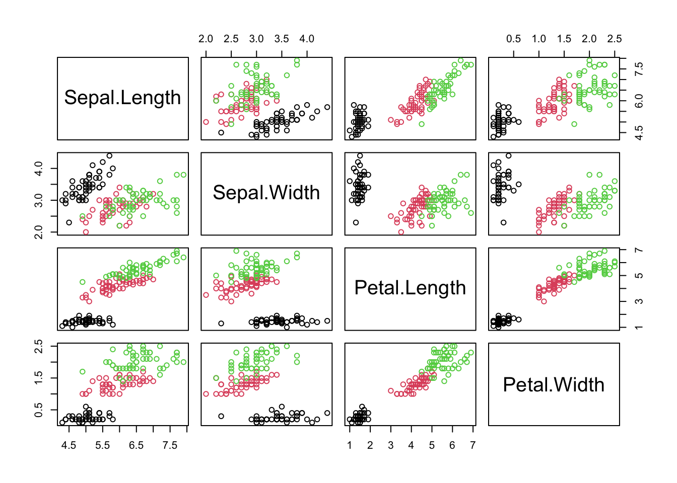
In this section, we use a simple example to demonstrate how to implement PCA with a simple program in R. First, we import the data, record some basic information, and visualize the data
dat = iris #import dataX =as.matrix(dat[,-5]) #take the 4 feature variables and save them in a matrixn =dim(X)[1] #record the sample sizep =dim(X)[2] #record the number of variablespairs(X, col = dat$Species) #visualize the data in a pairwise scatter plot
Next we do PCA on data matrix X. First, we calculate the covariance matrix.
S =cov(X) # calculate the covariance matrix
Second, do eigenvalue decomposition on covariance matrix S and save the results in res. In R, we can apply function eigen to perform eigenvalue decomposition.
res =eigen(S)str(res)
List of 2
 $ values : num [1:4] 4.2282 0.2427 0.0782 0.0238
 $ vectors: num [1:4, 1:4] 0.3614 -0.0845 0.8567 0.3583 0.6566 ...
 - attr(*, "class")= chr "eigen"
As shown above, the results of the eigenvalue decomposition contain all the information we need. slot values contains all the eigenvalues, and vectors contains all the eigenvectors, that is the optimal weights matrix.
W = res$vectors # define the weights matrix Ww_1 = W[,1] # the first column of W is the first PC weights.w_1
[1] 0.36138659 -0.08452251 0.85667061 0.35828920
Above, we define the weights matrix \(\textbf{W}\), and the first column, \(\textbf{w}_i\), contains the optimal weights for calculating the first extracted variables. Next, we extract the first PC of the first flower.
X[1, , drop = F]%*%w_1 # or, you can try sum(X[1,]*w_1) which is more like a weighted sum.
        [,1]
[1,] 2.81824
So, \(2.81824\) is just value of first PC for the first flower. We can extract the first PC for all the flowers together, then we get the first new variable.
z_1 = X%*%w_1
You can print out z_1 in your own computer and you will see it is a \(150 \times 1\) vector. We can even use matrix multiplication more efficiently to extract all possible principal components (PCs) at once.
Z = X%*%Wdim(Z)
[1] 150 4
You can see that the new data matrix Z has the same dimension as the original data matrix X. But what is the advantage of the new data matrix? We can find the answer by comparing the covariance matrices of the two data matrices.
It is easy to see that, compared to the original data matrix, the covariance matrix of the new data matrix is much simpler. The new variables are not only uncorrelated, but their variances gradually decrease.
This means that the amount of information contained in the variables of the new data matrix gradually decreases. The first new variable contains the most information, while the last new variable carries very little. Based on this, we can easily decide which variables to discard from the new matrix. This is the key essence of the PCA algorithm.
round(res$values,2)
[1] 4.23 0.24 0.08 0.02
Finally, let’s take a look at the eigenvalues obtained from the eigenvalue decomposition. Yes, the eigenvalues represent the variances of the new variables, which indicate the amount of information they contain.