3. Cross-Entropy Loss and Penalized Logistic Regression
3.1 Cross-entropy Loss and Likelihood function
Above, we conceptually explained the logistic regression model and its classifier and demonstrated its implementation in R. Next, we will address a more theoretical question: how to train our model, or in other words, how to estimate the model parameters. This question can be approached from both machine learning and statistical modeling perspectives, yielding consistent conclusions.
Strategy: From the machine learning perspective, it is relatively easy to formulate the optimization problem for the logistic regression model. However, different from MSE loss, to fully understand the cross-entropy loss function, we would need to learn some additional concepts from information theory. Since we have already studied likelihood theory, deriving the objective function (i.e., the likelihood function) from this perspective is comparatively straightforward. Therefore, to simplify the learning process, I will introduce the cross-entropy loss from the machine learning perspective and then interpret it through the lens of likelihood theory. In the near future, you can revisit this concept from the information theory perspective when you study neural networks.
3.1.1 Cross-entropy Loss
Let us recall the brute-force method we used when training a regression model. First, we define a loss function, specifically the MSE loss, which we use to evaluate the model’s performance.
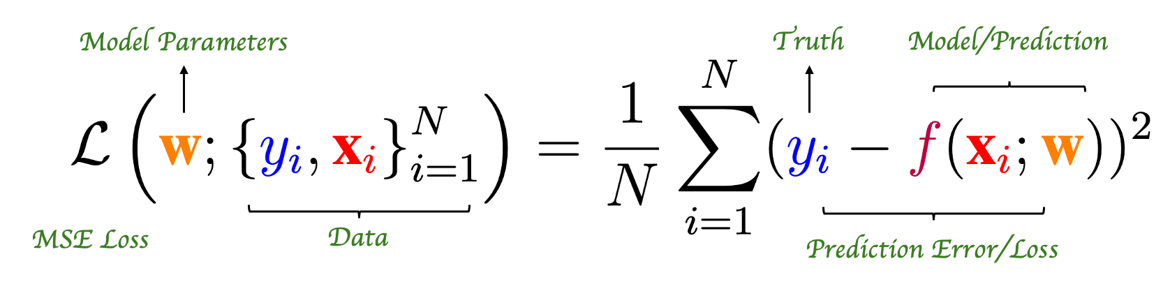
After defining the loss function, we can select the optimal model based on the performance corresponding to different sets of model parameters. In the absence of an efficient algorithm, brute-force computation is the simplest solution. However, for a well-defined optimization problem, smart mathematicians would never resort to brute-force computation so easily. This has led to the development of various algorithms for training models, e.g. gradient descent algorithm.
Alright, let’s return to the logistic regression model. How do we determine its model parameters? Similarly, we can design a loss function for the model and formulate it as an optimization problem. However, for a classification problem, we cannot directly calculate the model error and take the average, as we do in regression problems. Instead, the most commonly used loss function for classification problems is the cross-entropy loss: \[ \mathcal{L}\left(\textbf{w};\left\{ y_i, \textbf{x}_i \right\}_{i=1}^N \right) = -\frac{1}{N}\sum_{i = 1}^N \left\{ y_i\log( \pi(\textbf{x}_i, \textbf{w}) ) + (1-y_i)\log(1-\pi(\textbf{x}_i, \textbf{w})) \right\} \] Similar to training regression problems, the model parameters of logistic regression can be obtained by optimizing the cross-entropy loss, i.e., \[ \hat{\textbf{w}} = \arg\max_{\textbf{w}} \mathcal{L}(\textbf{w};\left\{ y_i, \textbf{x}_i \right\}_{i=1}^N) \]
Note: The cross-entropy loss is undeniably famous. You will encounter it again when you study neural network models and deep learning in the future.
Unlike regression problems, optimizing the cross-entropy loss does not have an analytical solution. This means that we must use numerical algorithms to find the optimal solution. Typically, we use second-order optimization algorithms to estimate the parameters of logistic regression, such as the Newton-Raphson algorithm you practiced in Lab 1. In broader fields, like optimizing deep neural network models, the gradient descent algorithm is commonly used. We will only touch on this briefly here, and I will discuss it in more detail in the future.
Think: Why can’t we design the loss function using prediction error like in regression problems? What would happen if we did?
3.1.2 Maximum Likelihood Estimation
Cross-entropy loss is not as easy to understand as MSE loss; you need to learn some information theory to fully grasp it. But don’t worry, here we will approach it from the perspective of statistical theory, specifically from the concept of maximum likelihood estimation (MLE), which you have already studied. In the end, you will find that the likelihood function of MLE and the cross-entropy loss are equivalent.
Suppose we have a set of training observations, \(\left\{ y_i, \textbf{x}_i \right\}_{i = 1}^N\). The distribution of the target variable is Binary distribution, i.e. \[ \Pr\left( y_i, \pi(\textbf{x}_i, \textbf{w}) \right) = \pi(\textbf{x}_i, \textbf{w}) ^{y_i} (1-\pi(\textbf{x}_i, \textbf{w}))^{1 - y_i} \] where \(y_i = 1 \text{ or } 0\). Since we have independent observations, the joint likelihood of the training sample is \[ L\left(\textbf{w}; ;\left\{ y_i, \textbf{x}_i \right\}_{i=1}^N \right) = \prod_{i = 1}^{n} \pi(\textbf{x}_i, \textbf{w}) ^{y_i} (1-\pi(\textbf{x}_i, \textbf{w}))^{1 - y_i} \] The log-likelihood function is \[ \ell\left(\textbf{w}; \left\{ y_i, \textbf{x}_i \right\}_{i=1}^N\right) = \sum_{i = 1}^N \left\{ y_i\log( \pi(\textbf{x}_i, \textbf{w}) ) + (1-y_i)\log(1-\pi(\textbf{x}_i, \textbf{w})) \right\} \] The MLE of \(\textbf{w}\) is \[ \hat{\textbf{w}}_{\text{MLE}} = \arg\max_{\textbf{w}} \ell\left(\textbf{w};\left\{ y_i, \textbf{x}_i \right\}_{i=1}^N\right) \]
Now we can compare the likelihood function and the cross-entropy loss function. Upon comparison, you will find that they differ only by a negative sign. Therefore, maximizing the likelihood function is equivalent to minimizing the loss function; they are interchangeable. So, if you want to understand cross-entropy loss, start by approaching it from the perspective of likelihood analysis.
3.2 Penalized Logistic Regression
In the previous lecture, we discussed the shrinkage and sparse versions of the regression model. Through these, we can both avoid the risk of overfitting and indirectly obtain feature selection results. For classification problems, we have similar tools available, that is penalized logistic regression.
Let’s first recall the idea of penalized regression. We define a set of candidate models by adding the calculation of the budget for the model parameter values, i.e., \[ \textcolor[rgb]{1.00,0.00,0.00}{\text{Candidate Models}} = \textcolor[rgb]{1.00,0.50,0.00}{\text{Full Model}} + \textbf{Budget}(\textbf{w}). \] With the general form of all candidate models, the penalized regression problem can be formulated as \[ \min_{\textbf{w}} \left\{ \mathcal{L}_{mse}\left( \textbf{w}; \left\{ y_i, \textbf{x}_i \right\}_{i=1}^N \right) + \lambda\textbf{Budget}(\textbf{w}) \right\} \] where the mse loss is just the sum squared residuals, and the budget term can be \(L_1\) norm, i.e. LASSO, or \(L_2\) norm, i.e. ridge regression.
Now, let’s return to the logistic regression model. The clever among you might have already realized that the difference between penalized logistic regression and the previous penalized regression is simply the choice of the loss function. If we replace the MSE loss in the above formula with the cross-entropy loss, we obtain the optimization problem for penalized logistic regression, and the optimal solution is the penalized logistic regression model parameters.
Similarly, if we choose the \(L_2\) norm, we will get a shrinkage solution, whereas the \(L_1\) norm will provide us with a sparse solution and serve as an important tool for feature selection in classification problems. In addition, we will encounter many variations of penalty terms, such as the Elastic net penalty, \[ \alpha \times \sum_{j = 1}^p |w_j| + (1- \alpha) \times \sum_{j = 1}^p w_j^2 \] where \(\alpha\) is an extra hyper-parameter taking value in \([0,1]\). From the above formula, it is easy to see that the calculation of the parameter value budget in elastic net is intermediate between ridge regression and LASSO. If the parameter \(\alpha\) is set to 1, the elastic net degenerates into the LASSO penalty. Conversely, if \(\alpha\) is set to 0, we get the \(L_2\) penalty, which corresponds to ridge regression. When \(\alpha\) takes any value between 0 and 1, we obtain the elastic net. In other words, the elastic net is a convex combination of the \(L_1\) penalty and the \(L_2\) penalty. This setup makes the corresponding candidate models more flexible. Of course, the trade-off is that we need to consider an additional hyperparameter. Alright, let’s stop here for now. We will explain the implementation of penalized logistic regression in more detail in the upcoming labs.