2. Logistic Regression Classifier
2. Logistic Regression Classifier
Do you know about logistic regression? It is an important tool in statistical analysis. In the future, I will write a note introducing it from a statistical perspective. Similarly, it is also one of the most important classifiers in machine learning. For now, let’s introduce logistic regression from a machine learning perspective.
2.1 Exploration
Let’s go back to our previous discussion: what is the main issue with using linear regression models for classification problems? First, we need to clarify one point: what is the essence of the linear regression model? Recall the discussion of maximum likelihood estimation of linear regression model. The essence of the linear regression model is to predict the expected value of the target variable using a linear combination of the feature variables, i.e. \[ \text{E}(y | \textbf{x}) = w_0 + w_1x_1 + w_2x_2 + \dots + w_px_p \] This is quite normal for a continuous target variable. However, when we try to extend this model to classification problems, we encounter new issues.
Essentially, we are trying to model the expected value of target variable as the weighted sum of feature variables, when we apply linear regression model to a classification problem. However, in classification problems, the target variable is a categorical variable. For categorical variables, the assumption of a normal distribution is completely unreasonable. We need to use discrete distributions to characterize the distribution of these variables, for example, using binary distribution for a binary classification problem, i.e. \(y \sim \text{Ber}(\pi)\), \[ y = \left\{ \begin{matrix} 1 & \text{Positive case} \\ 0 & \text{Negative case} \end{matrix} \right. \] What is the expected value of a binary distributed random variable? It is the probability of \(y = 1\), i.e. \(\text{E}(y) = \pi\). So, we are using the following equation \[ \pi|\textbf{x} = \text{E}(y|\textbf{x}) = w_0 + w_1x_1 + w_2x_2 + \dots + w_px_p \] If we analyze the range of values on both sides of the equation, it is not difficult to identify the critical flaw in using linear regression to handle classification problems. The left side of the equation represents a probability value, with a range of \([0, 1]\), while the right side can take any real number. Clearly, fitting a probability with an arbitrary real number is unreasonable and this is where the problem lies.
2.2 Model Construction
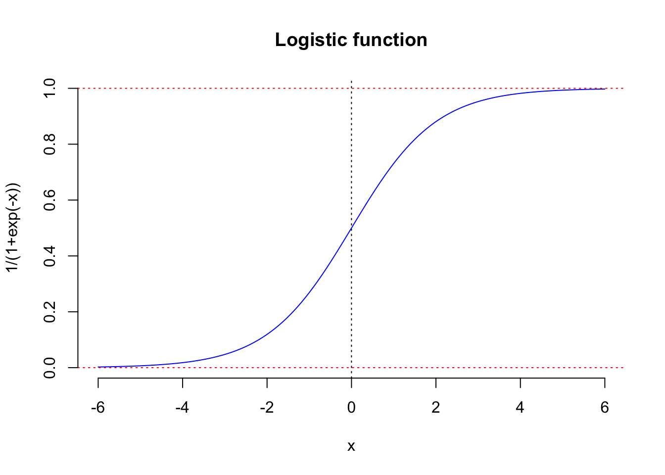
To address the issue mentioned above, mathematicians proposed an idea: using a function to transform values that span the entire real number axis into a fraction. This transformation function is the well-known logistic function, \[ \phi(t) = \frac{1}{1+e^{-t}} \] The graph of the logistic function is shown in the figure below. We can see that through its transformation, the output for any input \(x\) lies between the two red dashed lines, meaning it is a fraction.
With the help of the logistic function, we can start building our logistic regression model.
For a binary classification problem, we assume that the target variable follows a binary distribution, where the probability of a positive case is calculated as the logistic transformed weighted sum of the feature variables plus a constant. In a formal mathematical language, logistic regression model presents a probability model, \(y\sim \text{Ber}\left( \pi(\textbf{x}; \textbf{w}) \right)\), where \[ \pi(\textbf{x}; \textbf{w}) = \phi(w_0 + w_1x_1 + w_2x_2 + \dots + w_px_p) = \frac{1}{1 + e^{-(w_0 + w_1x_1 + w_2x_2 + \dots + w_px_p)}} \] As can be seen from the above model, the logistic regression model essentially provides us with a mechanism for calculating the posterior probability of the target variable, i.e. \[ \Pr\left( Y = 1 | \textbf{x} \right) = \frac{1}{1 + e^{-(w_0 + w_1x_1 + w_2x_2 + \dots + w_px_p)}} \] In other words, once we have obtained all the parameters \(\textbf{w}\), we can evaluate the posterior probability using the values of the feature variables. If you still remember the classification rule of the GDA classifier, \[ \widehat{y} = \arg \max_{y} \Pr(y| \textbf{x}) \] then it is natural that the logistic regression model can be used as a classifier. Simply speaking, if the posterior probability evaluated by logistic regression, \(\Pr\left( Y = 1 | \textbf{x}_{new} \right) > 0.5\), then we should classify this new case as positive, otherwise, negative group.
2.3 Logistic Regression in R
In R, we can apply glm function to estimate logistic regression model, and the usage is very simple.
# usage of function `glm` for estiamte logistic regression
model = glm(MODEL_EXPRESSION, family = binomial(), DATA)
Similar to using lm to estimate linear regression, we first need to specify the model expression, and the rules are the same. However, the difference is that we need to verify another argument, family, as Binomial. This argument mainly determines the type of the target variable \(y\), that is, it specifies its distribution. “Binomial” means that the target variable follows a binomial distribution, which implies that \(y\) has a binary distribution. More demonstration by examples will be presented in the next subsection.
Quiz: Can you guess what kind of model will be returned if you specify family as gaussian?
2.4 Decision Boundary
In the field of statistics, logistic regression is typically considered a type of generalized linear regression model. Generalized linear models (GLMs) form a large family of models, which includes common distributions for the response variable, such as Poisson regression, multinomial regression, beta regression, and so on. Logistic regression is also often referred to as a nonlinear regression model because, in the end, it projects the feature variables onto a nonlinear surface, as shown in the figure below.
LHS: Multivariate linear regression model. RHS: Logistic regression model, the surface is \(\phi(w_0 + w_1X_1+ w_2X2)\), where \(\phi\) is the logistic function.
Question: If logistic regression is considered a nonlinear statistical model, is it a nonlinear classifier?
R example:
Let’s address the previous example with outliers. To solve this problem, we can kill three birds with one stone: learn an R example, validate the robustness of logistic regression, and finally, experimentally obtain the answer to the above question.
I show you the dataset for the problem we discussed before and visualize it in a scatter plot.
head(dat) x1 x2 y
1 1.419 2.280 1
2 0.553 3.838 1
3 1.704 2.422 1
4 1.331 3.096 1
5 1.660 1.397 1
6 2.434 1.712 1color_obs = ifelse(dat$y==1, "blue", "red")
par(mar = rep(1,4))
plot(dat$x1, dat$x2, col = color_obs, pch = 20,
cex = 2, axes = F, xlab="", ylab = "")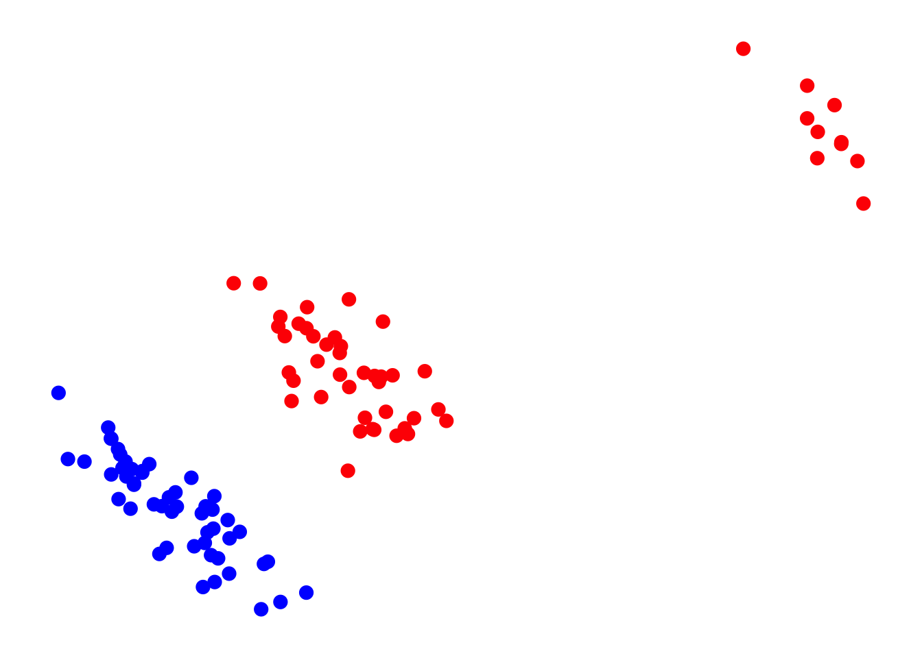
Let’s first demonstrate how to obtain the classification boundary for the linear regression model. By the way, the answer to the previous quiz is the linear regression model. That is, if we set the family argument to Gaussian, we will get a linear regression model. In other words, its output is the same as the output from the lm function. Now, let’s use it to calculate the model parameters.
m_linReg = glm(y~., data = dat, family = "gaussian")
summary(m_linReg)
Call:
glm(formula = y ~ ., family = "gaussian", data = dat)

Coefficients:
            Estimate Std. Error t value Pr(>|t|)
(Intercept)  1.08317    0.06386  16.962  < 2e-16 ***
x1          -0.03156    0.01510  -2.091   0.0392 *
x2          -0.10966    0.02241  -4.894 3.94e-06 ***
---
Signif. codes:  0 '***' 0.001 '**' 0.01 '*' 0.05 '.' 0.1 ' ' 1

(Dispersion parameter for gaussian family taken to be 0.1108737)

    Null deviance: 25.000  on 99  degrees of freedom
Residual deviance: 10.755  on 97  degrees of freedom
AIC: 68.805

Number of Fisher Scoring iterations: 2
Next, let’s render the classification boundary of the classifier based on this model. Similar to how we rendered the classification boundary for k-NN previously, we will first generate a grid for the 2D feature space. Then, we will use our model to classify each grid point and present the decision boundary.
x1 = seq(-1,16,0.1)
x2 = seq(0,14,0.1)
d = expand.grid(x1 = x1, x2 = x2)
class(d)
[1] "data.frame"scores = predict(m_linReg, d)
color_test = ifelse(scores > 0.5, "#D6E8FF", "#FFD6D6")par(mar = rep(1,4))
plot(dat$x1, dat$x2, col = color_obs, pch = 20,
cex = 2, axes = F, xlab="", ylab = "")
points(d$x1, d$x2, col = color_test, pch = 20, cex = 0.5)
points(dat$x1, dat$x2, col = color_obs, pch = 20, cex = 2)
As we observed earlier, the classifier based on the linear regression model is very sensitive to outliers. Even in such a simple classification problem, it makes errors in certain areas. Now, let’s take a look at the performance of the classifier based on the logistic regression model.
m_LogReg = glm(y~., data = dat, family = binomial())res_pred = predict(m_LogReg, d, type = "response")
range(res_pred)[1] 2.220446e-16 1.000000e+00Here, we use the predict function to predict the label for each grid point. Note that in the function above, we set the type argument to ‘response’, so we will obtain the posterior probability for each grid point based on its coordinates. Then, we can classify the points using the standard cutoff of 0.5. Finally, we use this grid to present the classification boundary of the classifier based on the logistic regression model.
color_test = ifelse(res_pred > 0.5, "#D6E8FF", "#FFD6D6")par(mar = rep(1,4))
plot(dat$x1, dat$x2, col = color_obs, pch = 20,
cex = 2, axes = F, xlab="", ylab = "")
points(d$x1, d$x2, col = color_test, pch = 20, cex = 0.5)
points(dat$x1, dat$x2, col = color_obs, pch = 20, cex = 2)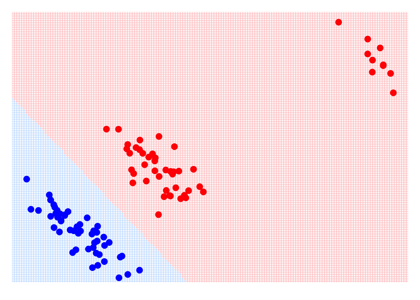
As we can see, using logistic regression as a classifier allows us to correct the impact of outliers. Additionally, we can observe that the classification boundary of the logistic regression classifier is also a straight line, meaning it is a linear classifier. In fact, this conclusion is not difficult to reach. From the principle of the classifier, the classification boundary of the logistic regression classifier is: \[ \Pr(Y = 1|\textbf{x}) = \phi(\text{scores}) = \frac{1}{1 + e^{-(w_0 + w_1X_1 + \dots + w_pX_p)}} = \frac{1}{2} \] If we simplify this formula, we can derive the classification boundary of the logistic regression classifier \[ w_0 + w_1X_1 + \dots + w_pX_p = 0 \] So, the classifier based on logistic regression is a linear classifier.