5. Regression Model and Classification Model
5.1 Regression Model
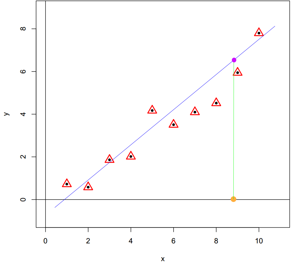
The machine learning problem can be understood as regression problem when the target variable is a continuous variable. For example, predict the house price based on different feature variables; predict the pixel values of CT scans based on MRI scans; predict the stock price based on feature variables of market. A simple scenario displayed in the figure below, a basic regression model is a linear model, \(y_i = w_0 + w_1x_i + \epsilon_i\). From a geometric perspective, a linear regression model can be seen as a straight line that passes through all sample observations. In the generalization stage, the target value can be predicted from feature variable through the regression model.
5.2 Classification Model
The problem can be viewed as a classification problem when the target variable is categorical. We often refer to this type of target variable as labels. For example, in the classification with Iris data, the species variable is the label variable, and we aim for finding a good “function” taking 4 shaping variables as input to predict the labels based on data. This function is often refer to a classifier. So, what kind of function can perform this role? Let’s take a look at a real classifier first, a “coin sorter.” Its operation is quite simple, as it classifies coins based on their different diameters. Inside the machine, there are holes of varying sizes corresponding to different diameters, and through vibration, coins will fall into the holes that match their size. In essence, it’s classifying by comparing a variable to a threshold value. The idea is quite simple, but it is just the essential idea of machine learning classifier.

Well, usually we have multiple feature variables in a classification problem, then how do we apply this simple working principle to design a classifier? Let’s see another example. You might not know yet, in fact, teacher becomes a classifier after an exam. Well, to pass or not to pass is a classification problem. Suppose, in a secret exam, each student answers 5 questions and each question is worth 20 points. Student passes the exam if the total points are larger or equal to 60. I have corrected all the exams; the results are summarized in Table 1, and \(1\) indicating the question was correctly answered and \(0\) indicating not. Then, who can pass the exam?
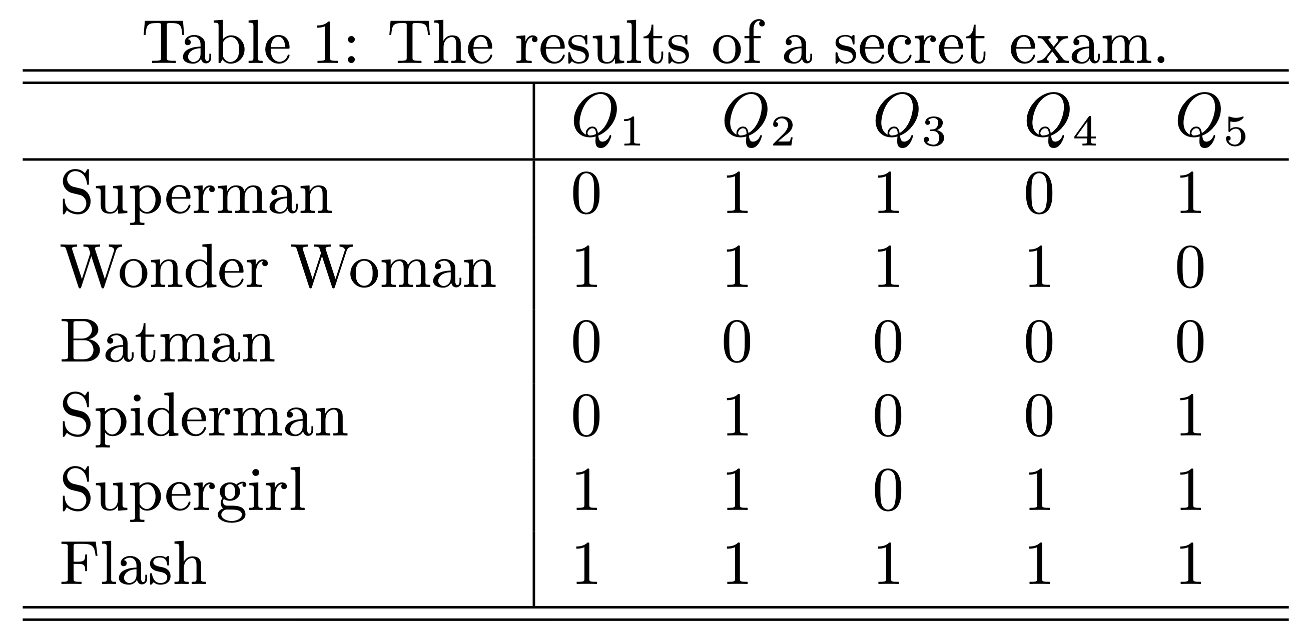
I believe it is a very simple problem, for example, Super girl correctly answered 4 questions and get 80 points that is above the threshold value 60, so she passed the exam! However, spiderman only got 20 points that is lower than 60, so he can’t pass. If we clearly write down the calculation process, we actually used the following formula to calculate the totol score, then compare the total score with the critical point, 60.
\[ 20\times Q_1 + 20\times Q_2 + 20\times Q_3 + 20\times Q_4 + 20\times Q_5 \geq 60 \]
Now, we know what a simple classifier looks like. Essentially, it is a two-step procedure. We create a single variable through the weighted sum of all feature variables first, then compare the resulting value with a threshold value. In formal, the classifier can be represented as
\[ y = \text{Sign}(w_0 + w_1 x_1 + w_2 x_2 + \dots + w_p x_p) \]
where \(\text{Sign}(x)\) is a sign function returning 1 if \(x>0\) and 0 if \(x<0\). We refer coefficients \(w_1, \dots, w_p\) as weights, the weighted sum of feature variables \(w_1 x_1 + w_2 x_2 + \dots + w_p x_p\) as scores and \(w_0\), the threshold value, as bias. If the score value is equal to 0, then this observation can’t be classified by this classifier, and the thing we can do best is flip a coin to make the decision. We call all the points that satisfy equation \(w_0 + w_1 x_1 + w_2 x_2 + \dots + w_p x_p = 0\) as the decision boundary. For example, in a 2D feature space, the decision boundary \(w_0 + w_1x_1 + w_2x_2 =0\) is just a straight line with a slope of \(-w_1/w_2\) and an intercept of \(-w_0/w_2\), see the figure below.
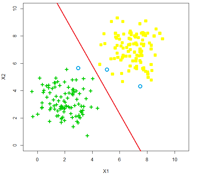
This kind of classifier is called linear classifier, since the decision boundary is presented by a linear function. It is a straight line in 2D space, a plane in 3D space, and hyper-plane in a higher dimension space. You might have already realized that in fact, a classifier is solely determined by its weights and bias, and machine learning algorithms tell us how to find the optimal weights and bias through data. There are several classical methods (algorithms) for learning a linear classifier which are perceptron algorithm, linear discriminant analysis, logistic regression, and maximum margin classifier. In this course, we will introduce all of them except maximum margin classifier.
Remark: Just as all the rules of arithmetic start with \(1+1\), don’t underestimate this linear classifier. You will see that all complex classifiers are built upon them. For example, maximum margin classifier is the foundation of SVM (Support vector machine) which dominate machine learning world for 20 years, the perceptron algorithm is the starting point of artificial neural net works, and no matter how complex a neural network architecture may be, as long as it is a classifier, its final layer will inevitably be a logistic regression model.
