Cracking the Code

A real example of problem solving with data

In this note, we discuss a cryptography problem introduced by Prof. Persi Diaconis in his paper, see [1]. He used this example to illustrate the Markov Chain Monte Carlo (MCMC) approach. This example is not only an elegant introduction to MCMC but also a great demonstration of the “routine” of using data to solve real-world problems. Additionally, it provides an opportunity to review fundamental probability concepts and serves as a valuable programming exercise—you may even try implementing it yourself.

The story takes place in a U.S. prison. One day, a police officer discovered a piece of paper covered in strange symbols (see the figure below). It turned out that some prisoners were attempting to exchange secret messages using a cipher. The officer first consulted a linguist, who suggested that the ciphertext might be a simple substitution cipher. Unable to decipher it themselves, the linguist recommended seeking help from statisticians.

Problem Understanding

First of all, let’s understand what is a substitution cipher. It is a very simple cipher using fixed symbols to replace letters, punctuation marks, numbers, and spaces. Then the key of this kind of cipher is a map from the symbol space to the letter space.

\[ f: \{ \text{code space} \} \to \{ \text{alphabet} \} \]

We use the letter itself instead of symbols to simplify the problem and make it easier to express. For example, suppose the key is

\[ f: \{ \text{d} \to \text{a}, \text{a} \to \text{t}, \text{t} \to \text{d}, \dots \} \]

According to this key, the regular English word “data” is encrypted as “atdt”. Next, same as the original paper, we take a small piece from the well-known section of Shakespeare’s Hamlet as a simple example.

enter hamlet ham to be or not to be that is the question whe ther tis nobler in 
the mind to suffer the slings and arrows of outrageous fortune or to take arms against 
a sea of troubles and by opposing end.

We randomly generate a substitution cipher:

tuntvmfeprtnmfepmnsmgtmsvmusnmnsmgtmnfenmjbmnftmatbnjsumdftnftvmnjbmusgrtv 
mjumnftmpjuymnsmbiitvmnftmbrjuhbmeuymevvsdbmsims nvehts bmisvn 
utmsvmnsmnextmevpb mehejubnmembtemsimnvs g rtbmeuymgwmskksbjuhmtuy

One can apply an inverse mapping to decrypt the cipher and retrieve the hidden message. In other words, if one holds the key, the cipher becomes understandable. Thus, the challenge is to determine the key (mapping \(f\)). However, this is far from an easy task, because the symbol space is too large for a brute-force search to be feasible. Even if we only consider lowercase letters and spaces, the total number of possible keys is \(27! = 1.08 \times 10^{28}\). Given this immense complexity, we need a smarter approach—one that incorporates prior information to guide the search. This prior knowledge forms the foundation of our assumptions and the model built upon them.

Model and Assumption

For a natural language, we believe the alphabetical order should obey certain rules. For example, the probability of the letter ‘a’ being connected by the letter ‘b’ must be greater than that of the letter ‘x’. Now we translate this prior knowledge as an assumption. To do so, we view the sequence of letters in a text as a stochastic process. There could be \(27\) possible values for each time point (or position). We call the possible values (letters) as state. Then we can assume that a sequence of letters in a text should satisfy the first-order Markov properties.

\[ \Pr(x_t | x_{1}, x_{2}, \dots, x_{t-1}) = \Pr(x_t | x_{t-1}) \]

where \(x_i\) present the state at the \(t\)-th position in a text. In other words, the letter in \(t\)-th position only depends on the letter in the previous position. This assumption implies two things. First, the transition between two letters in a text should satisfy some transition probabilities and this can be summarized in a transition probability matrix,

\[ \begin{pmatrix} & a & d & t & \dots \\ a & p_{11} & p_{12} & p_{13} & \dots \\ d & p_{21} & p_{22} & p_{23} & \dots \\ t & p_{31} & p_{32} & p_{33} & \dots \\ \vdots & \vdots & \vdots & \vdots & \ddots \end{pmatrix} \]

The second thing is the likelihood of a text can be factorized as the product of the corresponding transition probabilities. For example, the likelihood of ‘data’ is

\[ \ell('data') = \Pr(d\to a)\Pr(a\to t)\Pr(t\to a) = p_{21}p_{13}p_{31}, \]

but the likelihood of ‘atdt’ is

\[ \ell('atdt') = \Pr(a\to t)\Pr(t\to d)\Pr(d\to t) = p_{13}p_{32}p_{23}. \]

Since ‘atdt’ is much weirder than ‘data’, the likelihood of the former must be lower than the latter, \(\ell('atdt') < \ell('data').\) Given the two thoughts, we can summarize our problem as an optimization problem and present it in a mathematical language,

\[ \max_{f} \ell( f( \text{Cipher}) ) \]

So the problem is to find a key \(f\) that maximizes the likelihood of the translated text, \(f(\text{Cipher})\). Great! We have obtained a promising idea, however, it is still not clear how to search for the key in a smart way. Before we discuss the final solution, we need to first discuss one practical issue, that is how to obtain the transition probability matrix.

Model Estimation

At this stage, we can finally invite our protagonist, data. So far, we have a probability model, the first-order Markov chain model. It is a parametric model and the parameter is the transition probability matrix. To be a little bit mysterious, we can’t know the real model coefficients set by God, we can only try to figure out his mind through the data generated by the model he created. Seriously speaking, we need to use the data to estimate the parameters of the model. For this problem, we can download classical books in English and that is our data. More specifically, we can count the frequencies of all \(27^2\) different transitions in a book. Then normalize all the frequencies by the total number of transitions as the estimation of the transition probabilities. You can see part of the estimation of the transition probability matrix bellow

\[ \begin{matrix} & A & B & C & D & E & F & G & H & I & \dots \\ A & 0.000 & 0.017 & 0.034 & 0.055 & 0.001 & 0.008 & 0.017 & 0.002 & 0.043 & \dots \\ B & 0.093 & 0.007 & 0.000 & 0.000 & 0.328 & 0.000 & 0.000 & 0.000 & 0.029 & \dots \\ C & 0.110 & 0.000 & 0.017 & 0.000 & 0.215 & 0.000 & 0.000 & 0.184 & 0.042 & \dots \\ D & 0.021 & 0.000 & 0.000 & 0.011 & 0.116 & 0.001 & 0.004 & 0.000 & 0.066 & \dots \\ E & 0.042 & 0.001 & 0.017 & 0.091 & 0.026 & 0.010 & 0.007 & 0.002 & 0.011 & \dots \\ F & 0.071 & 0.001 & 0.000 & 0.000 & 0.084 & 0.052 & 0.000 & 0.000 & 0.085 & \dots \\ G & 0.066 & 0.000 & 0.000 & 0.001 & 0.115 & 0.000 & 0.009 & 0.117 & 0.049 & \dots \\ H & 0.164 & 0.000 & 0.000 & 0.000 & 0.450 & 0.000 & 0.000 & 0.000 & 0.156 & \dots \\ I & 0.017 & 0.008 & 0.049 & 0.050 & 0.049 & 0.022 & 0.025 & 0.000 & 0.001 & \dots \\ \vdots & \vdots & \vdots & \vdots & \vdots & \vdots & \vdots & \vdots & \vdots & \vdots & \ddots \end{matrix} \]

Once the transition probability is ready, then we can use it to evaluate the likelihood of a text. For example, the likelihood of the original text and the cipher is \(-458.26\) and respectively.

Inference

Great! Now we can discuss how to find the optimal key. Imagine that all the \(27!\) possible keys form a huge solutions space. Similar to most optimization algorithms, we can start from a certain initial value, and then gradually approach the optimal solution through some iterative mechanism. (In fact, this is not very accurate, but we can understand it this way first, and later I will explain what our algorithm is doing.) Firstly, we randomly generate an initial key, for example

\[ f^{(0)}: \{ \text{a} \to \text{f}, \text{b} \to \text{g}, \text{c} \to \text{m}, \dots \}, \]

and evaluate the likelihood of this key \(\ell(f^{(0)}(cipher))\). Then we randomly move a small step to a new key \(f^{(1)}\) by making a random transposition of the values \(f^{(0)}\) assigned to two symbols, for example,

\[ f^{(1)}: \{ \text{a} \to \text{m}, \text{b} \to \text{g}, \text{c} \to \text{f}, \dots \} \]

Is the new \(f^{(1)}\) key a good proposal? We can calculate its likelihood value and compare it with the previous key. The simple situation is that if the likelihood value of the decoded text with the new key is higher than the previous one, \(\ell(f^{(1)}) > \ell(f^{(0)})\), we should keep the new key. The interesting question is what if the new key is worse? Simply discard this new key? It seems to be a good way, but there is a risk of falling into the local area and finally missing the optimal key. What is the good way then? There are two situations. If the likelihood value of the decoded text with the new key is much lower than the previous key, then we should be inclined to abandon it; however, if the likelihood values of the two keys are almost the same, then we should tend to keep it. This plan sounds more reasonable, but the question is how exactly realize ‘tend to’? We can calculate the ratio, \(\frac{ \ell(f^{(t)}) }{ \ell( f^{(t-1)}}\). First, this value is a decimal number between 0 and 1. Second, if the likelihood of the text decoded with the new key is significantly lower than that of the text decoded with the old key, then this decimal will be very close to 0. Conversely, it will be a decimal very close to one. So, it can be regarded as a probability that an action will be executed. If we generate a Bernoulli-distributed random number with this probability, and use it to determine whether to keep the new key, then the above operation can be achieved. We summarize this approach in the following algorithm

Initialize the key f(0)
for(i in 1:R){
  Step 1. Evaluate the likelihood value of f(t-1), likelihood(f(t-1))
  Step 2. Propose a new key f(t) by making a random transposition of the values of f(t-1) assigned to two letters.
  Step 3. Make decision, either keep the new key or stay with the old key
  if(likelihood(f(t)) > likelihood(f(t-1))){
    keep f(t)
  } else{
    generate u ~ Ber(likelihood(f(t))/likelihood(f(t-1)))
    if(u == 1){
      keep f(t)  
    } else{
      stay at f(t-1)
    }
  }
}

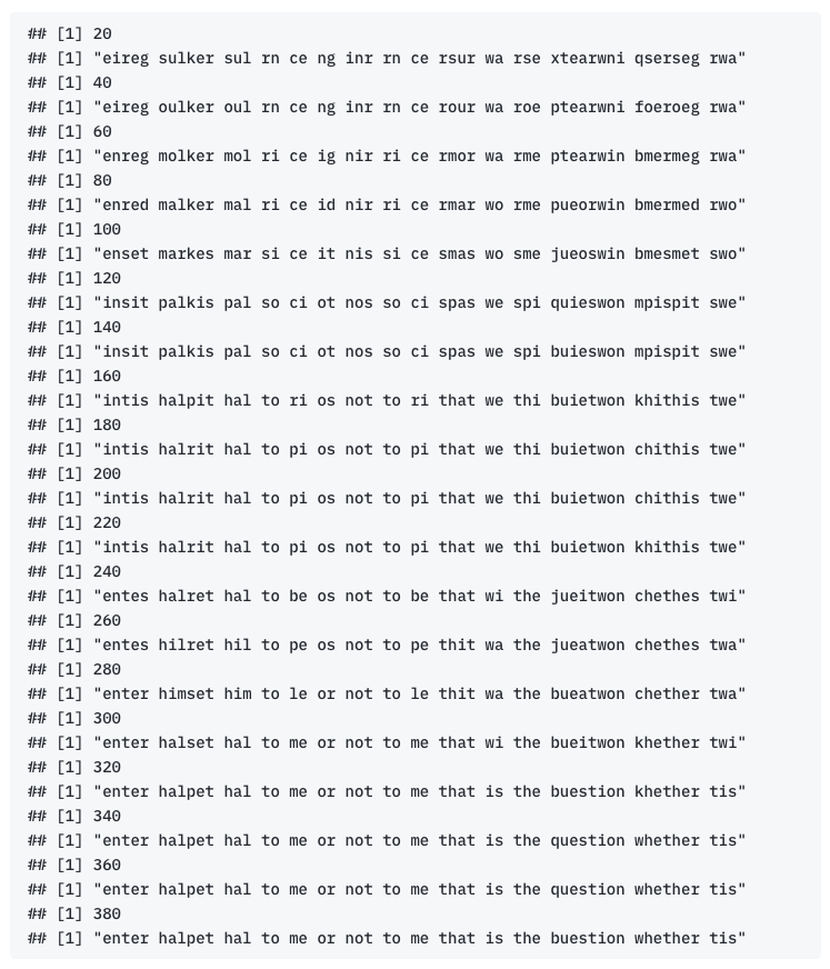
The performance of our algorithm can be glimpsed from the following R outputs.

Reference：

[1] Diaconis, Persi. “The markov chain monte carlo revolution.” Bulletin of the American Mathematical Society 46.2 (2009): 179-205.