Task 3: Deep ANN model

In this exercise, we attempt to train a neural network model with two hidden layers to solve a multiple-class classification problem. We use the famous MNIST dataset for this task. Although it contains a large number of labeled samples—70k in total for training and testing—the relatively high resolution of the images, \(28 \times 28\), requires us to apply additional techniques to prevent overfitting.

Step 1: Prepare Data

This dataset is already included in the Keras package, so you can directly obtain the data using the following code:

mnist = dataset_mnist()
x_tr = mnist$train$x
g_tr = mnist$train$y
x_te = mnist$test$x
g_te = mnist$test$y

Next, we need to preprocess the data. First, the pixel values of the images range from 0 to 255. To improve training performance, we need to normalize them.

x_tr = x_tr/255
x_te = x_te/255

The following chunk of codes are recommended for visulazing the images.

# visualize the image
library(jpeg)
par(mar = c(0,0,0,0), mfrow = c(5,5))
id <- sample(seq(50000), 25)
for(i in id){
  plot(as.raster(x_tr[i,,]))
}

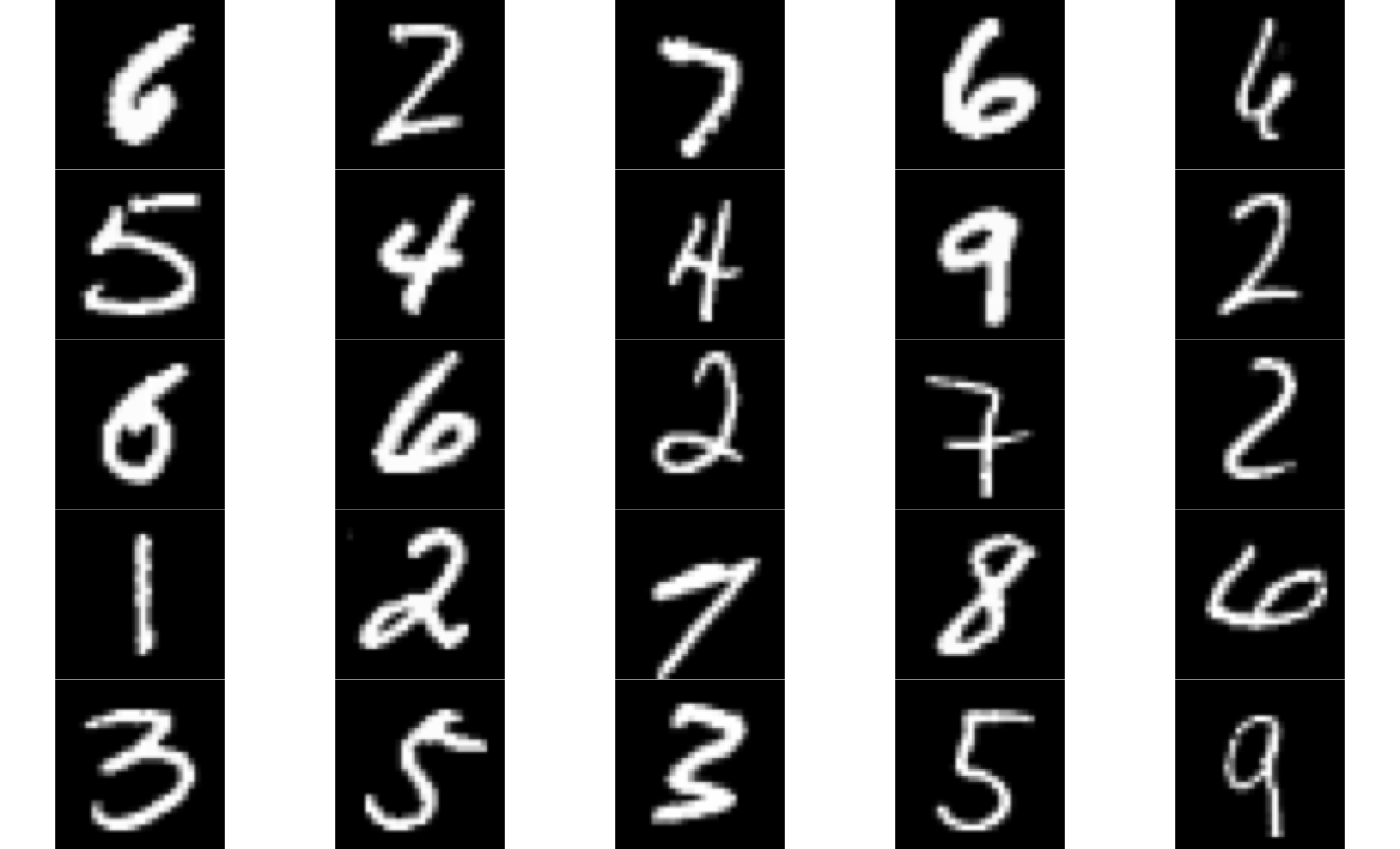
First, unlike the HWD dataset we used earlier, each image in this dataset is stored in matrix form. Therefore, we need to reshape all the image data.

x_tr = array_reshape(x_tr, c(nrow(x_tr), 784))
x_te = array_reshape(x_te, c(nrow(x_te), 784))

Finally, since this is a multi-class classification problem, we need to encode the integer target variable by function to_categorical.

y_tr = to_categorical(g_tr, 10)
y_te = to_categorical(g_te, 10)

Now the data is ready!

Step 2: Draw the model

Next, we can use keras_model_sequential() to assemble our neural network model. Below is the recommended model architecture. A few points need to be noted:

Since the model has multiple layers, we use ReLU as the activation function.
As mentioned earlier, we need some techniques to control overfitting. Here, we can use the dropout method. In Keras, we use the layer_dropout() function to implement this.

ANN_mod = keras_model_sequential() %>%
  layer_dense(units = 256, activation = "relu", input_shape = c(?)) %>%
  layer_dropout(rate = 0.4) %>%
  layer_dense(units = 128, activation = "relu") %>%
  layer_dropout(rate = 0.3) %>%
  layer_dense(units = 10, activation = "?")

Note: The question marks in the code require your judgment and modification.

Step 3: Compile the model

Next, we can compile our model. Please check which loss function we need. Additionally, we choose RMSprop as our optimization algorithm.

ANN_mod %>% compile(loss = "?", 
                    optimizer = optimizer_rmsprop(),
                    metrics = c("accuracy"))

Step 4: Train the model

Now, we begin training the model. Here, we introduce a new argument, validation_split, which is mainly used to split a portion of the training data to be used as validation data during training. This helps in monitoring the model’s performance on unseen data and can help detect overfitting during training.

Training_history = ANN_mod %>% 
  fit(x_tr, y_tr, repochs = 30, batch_size = 128, validation_split = 0.2)

Prediction

Finally, let’s take a look at the performance of the trained model on the test set.

predict <- predict_classes(mod_1, x_te)
head(y_te)
g_te
mean(predict == g_te)
table(predict, g_te)

Previous page | Lecture 3 Homepage | Next page