Solutions to Lab 1

Task 1: Image reconstruction

In the next series of tasks, we implement image reconstruction with HWD dataset.

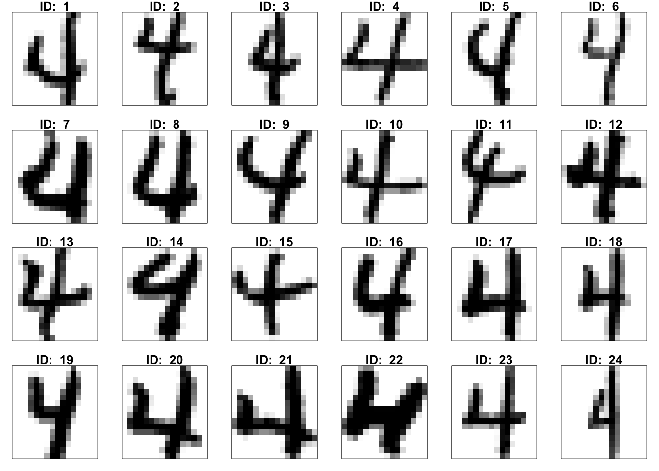
Task 1.1: Choose your favorite number. Use the function ‘image’ to display the first 24 cases. Below is an example of the usage method for the function image(). In the following R chunk, the first two lines are about color settings. You can also try your favorite color palette. In the third line, X represents all images of your favorite number, which refers to the part of the Dat matrix in R space excluding the first column. The last line generates the plot of the 8th image in X.

colors = c('white','black')
cus_col <- colorRampPalette(colors=colors)
temp = matrix(X[8,256:1],16,16,byrow=T)[,16:1]
image(t(temp), col=cus_col(256), frame = T, axes = F)

Choose all the images of my favorite number:

X = dat[which(dat[,1] == 4), -1]
dim(X)

[1] 652 256

Visualize the first 24 images in the dataset by using function image()

colors = c('white','black')
cus_col <- colorRampPalette(colors=colors)

par(mfrow = c(4,6), mar = rep(1,4))
for(i in 1:24){
  temp= matrix(X[i,256:1],16,16,byrow=T)[,16:1]
  image(t(temp), col=cus_col(256), frame = T, axes = F)
  title(paste("ID: ", i))
}

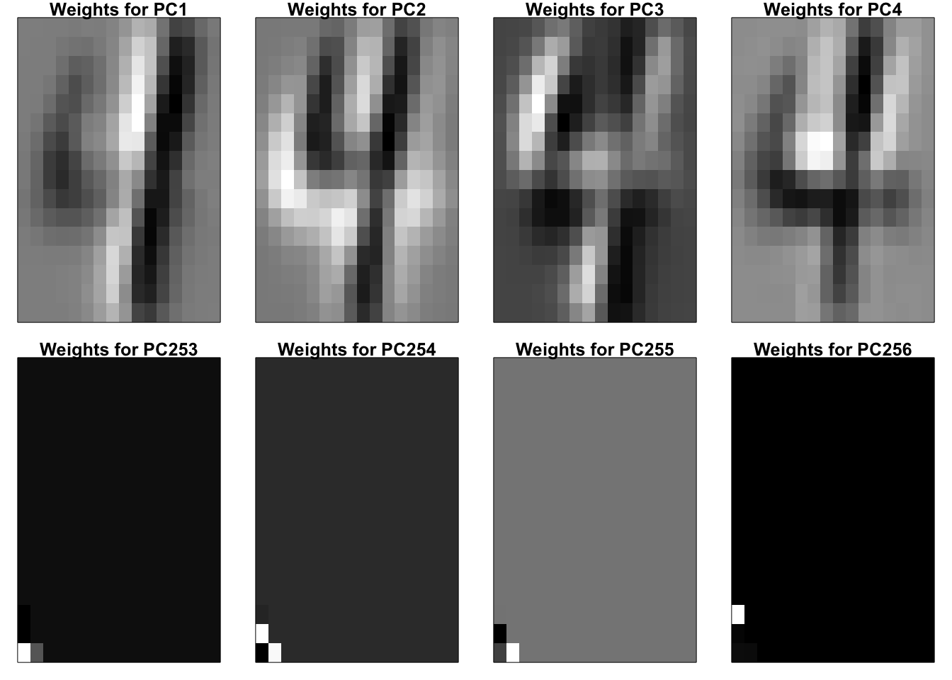
Task 1.2: Do PCA on your data set. Display the first 4 and the last 4 principal vectors (eigenvectors) as \(16 \times 16\) images.

To do PCA, we first calculate the covariance matrix of X, then do eigenvalue decomposition on the contrivance matrix.

S = cov(X)
res = eigen(S)
W = res$vectors

All the PC weights are saved in W; each column is a set of weights for calculating the corresponding new variable, PC. Next, we display the first 4 and the last 4 columns of W as images.

par(mfrow = c(2,4), mar = rep(1,4))
for(i in c(1:4, 253:256)){
  temp = matrix(W[256:1,i],16,16,byrow=T)[,16:1]
  image(t(temp), col=cus_col(256), frame = T, axes = F)
  title(paste0("Weights for PC", i))
}

Task 1.3: Calculate all the PCs for all the images of your favorite number.

If you are familiar with matrix calculations, then you can get the new data matrix directly

Z = X%*%W
dim(Z)

[1] 652 256

Otherwise, you can calculate all the PCs for all the image by a double for lop.

n = dim(X)[1]
Z = X
for(i in 1:n){
  for(j in 1:256){
    Z[i, j] = sum(X[i,]*W[j])
  }
}

Task 1.4: Image reconstruction. Reconstruct an image in your data set by its first 30, 60, 100, 150, and 200 principal components separately. Put the original image and five approximated images in one plot. For each approximated image, calculate and report the mean square errors.

This also can be done by matrix calculation. However, we will do it by for loop first since it is more understandable. Next, I will reconstruct the 8th image of number 4.

k = 150 # we use k PCs to reconstruct the image
x_hat = Z[8,1]*W[,1]
for(i in 2:k){
  x_hat = x_hat + Z[8,i]*W[,i]
}
# vis
par(pin = c(4, 4))
temp = matrix(x_hat[256:1],16,16,byrow=T)[,16:1]
image(t(temp), col=cus_col(256), frame = T, axes = F)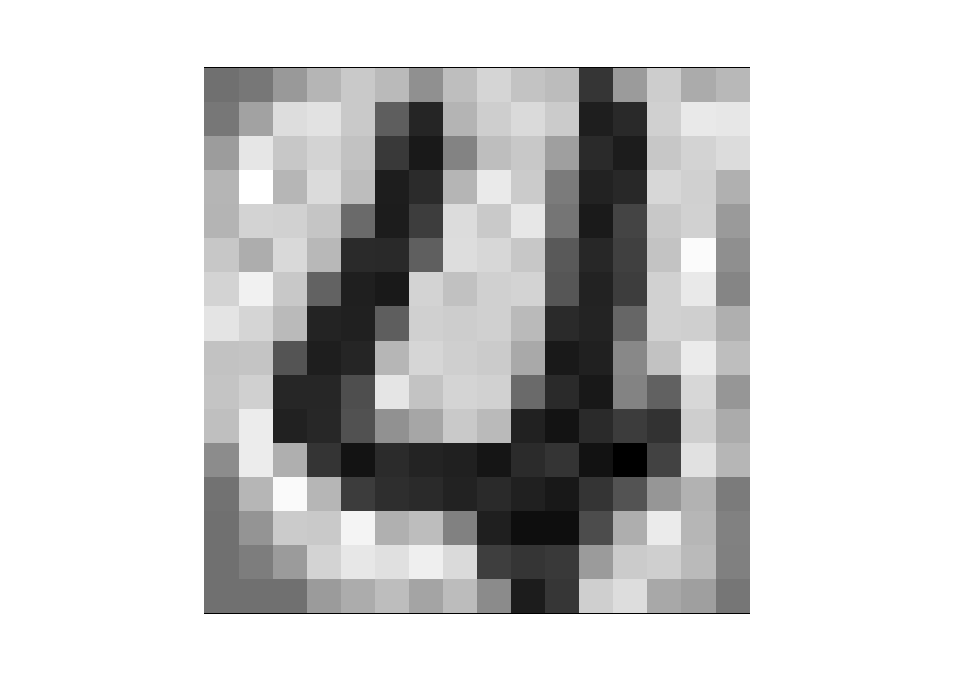

The approximation error is

mean((X[8,]-x_hat)^2)

[1] 0.0904779

You can get the same results by matrix multiplication.

par(pin = c(4, 4))
temp = W[,1:30]%*%t(Z[8,1:30,drop = F])
temp = matrix(temp,16,16,byrow=T)[16:1,]
image(t(temp), col=cus_col(256), frame = T, axes = F)

Task 2: Train a classifier with extracted features

Build a classifier based on the first two principal components (PCs) to classify the images of digits 5 and 6. The following procedure is suggested to solve this task.

Create a new working dataset that contains all the images of 5 and 6.
Split the data set into training set (\(80\%\)) and testing set (\(20\%\)) by random sampling.
Do PCA on the training set. Use the eigenvectors of the sample covariance matrix of the training set to calculate the PCs for both the training set and testing set.
Use PCs of the training set to build the classifier
Apply your classifier to the testing set PCs and calculate the accuracy.

Step 1:

X = dat[which(dat[,1] %in% c(5,6)), -1]
y = dat[which(dat[,1] %in% c(5,6)), 1]

Step 2:

n = dim(X)[1]
set.seed(2025)
id = sample(1:n, 0.8*n)
X_tr = X[id, ]
y_tr = y[id]
X_te = X[-id, ]
y_te = y[-id]

Step 3:

S = cov(X_tr)
W = eigen(S)$vectors

Z_tr = X_tr%*%W[,1:2] 
Z_te = X_te%*%W[,1:2]

par(mfrow = c(1,2))
plot(Z_tr, col = y_tr)
plot(Z_te, col = y_te)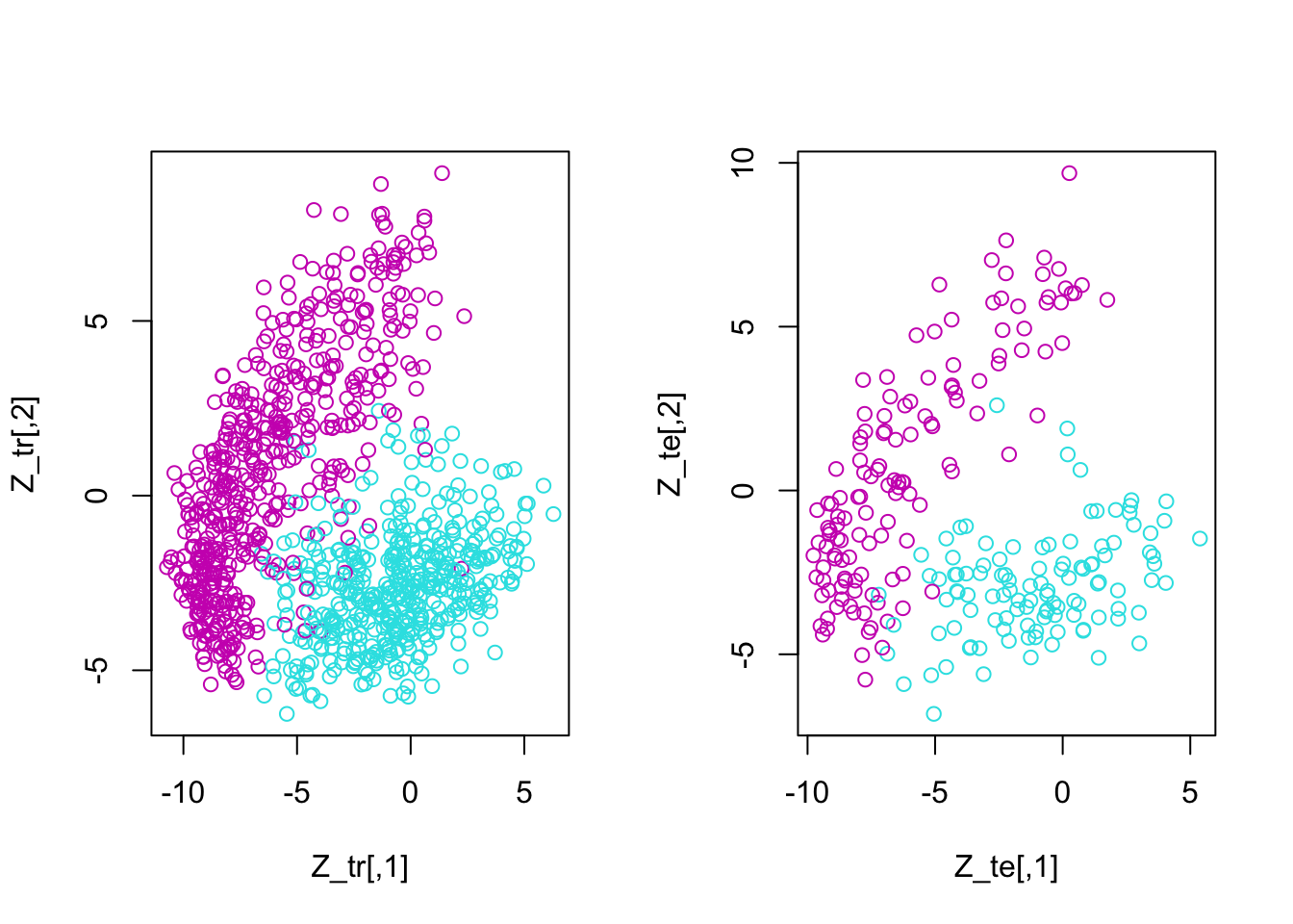

par(mfrow = c(1,1))

Step 4:

d_tr = data.frame(y = ifelse(y_tr == 5, 1, 0), z1 = Z_tr[,1], z2 = Z_tr[,2])
head(d_tr)

  y         z1         z2
1 1 -5.2767511 -4.9867831
2 0 -8.3540556 -4.3457323
3 0 -2.1933222  3.4651025
4 0 -2.7204058 -0.3158707
5 1 -0.5886785 -3.9040087
6 0 -7.7362370 -0.4245627

m = glm(y~z1+z2, family = binomial(), data = d_tr)
w = m$coefficients
par(mfrow = c(1,2))
plot(Z_tr, col = y_tr)
abline(-w[1]/w[3], -w[2]/w[3])
plot(Z_te, col = y_te)
abline(-w[1]/w[3], -w[2]/w[3])

par(mfrow = c(1,1))

Step 5:

d_te = data.frame(y = ifelse(y_te == 5, 1, 0), z1 = Z_te[,1], z2 = Z_te[,2])
res = predict(m, d_te, type = "response")
y_pre = ifelse(res > 0.5, 1, 0)

mean(y_pre == d_te$y)

[1] 0.954918

table(y_pre, d_te$y)

     
y_pre   0   1
    0 129   8
    1   3 104

Can you achieve this level of accuracy using only two variables from the original dataset to build the classifier? Think about it.

Lecture 2 Homepage