Lecture 7: Logistic Regression Classifier
In this lecture, we will learn about a very important classifier in machine learning, the logistic regression classifier. First, we will discuss intuitively how classification can be performed using a linear regression model and point out its critical weakness. Then, we will introduce logistic regression to address this weakness, discussing its model construction and how to use it as a classifier. Finally, we will discuss the training of the logistic regression model. By understanding its loss function, we will easily grasp how to use regularization methods in logistic regression.
1. Regression Model for Classification
“Regression model for classification” sounds a bit strange. Do these two types of problems have something in common? How can we use a linear regression model to build a classifier?
1.1 Motivation
As we discussed earlier, if there is only one feature variable, how can we perform classification? Let’s revisit this simple problem to gain some insights. Based on our previous discussion, the key to this problem lies in determining the classification boundary, that is, finding a method to identify the cutoff. For example, when discussing Fisher’s idea, we mentioned that for two normal distributions with equal variance, the optimal classification boundary is the midpoint between the two population means. Now, let’s approach this from a different perspective.
The difficulty of this problem lies in the fact that different feature variables will have different criteria. For example, we might use body size to distinguish between ethnic groups, flower shape measurements to classify flower species, or image-extracted features to diagnose cases. However, there is no universal cutoff to serve as a standard for all of them. Therefore, we need to transform any variable onto a dimension that has a universal cutoff. So, which dimension is that magical dimension, and what should we do to find it?
We can use the target variable to find the magical dimension to perform the transformation. First, we encode the target variable to make the categorical variable numerical—for example, assigning 1 to the positive group and 0 to the negative group. Then, we estimate a linear regression model for the target variable based on the feature variables. Through the regression model, all observation points are projected onto that magical dimension, where 0.5 serves as the universal cutoff. See the demo below:
Remark: You might find this problem a bit tedious and think, “Why not just pick a random point in the region between the two populations?” However, note that this approach is overly subjective. What we need is a universal method to calculate this cutoff, such as Fisher’s idea or the method discussed here. In the future, we will introduce a third approach. You can also think about whether you have any good ideas.
1.2 Classifier based on Linear Regression Model
This idea can be naturally extended to the case of multiple feature variables. Suppose we have a set of feature variables, \(X_1,X_2,\dots,X_p\), and the encoded target variable \(Y\). The trained multivariate linear regression model is \[ Y = w_0 + w_1X_1 + w_2X_2 + \dots + w_pX_p \] With this model, the \(p\) feature variable values of any observation are recalculated and used for the final decision. We call the fitted \(Y\), \(w_0 + w_1X_1 + w_2X_2 + \dots + w_pX_p\), Score. So, if \(\text{Score} > 0.5\) then it will be assigned as positive, and if \(\text{Score} < 0.5\) then it will be assigned as negative. So the decision boundary will be \(\text{Score} = 0.5\), i.e. \[ w_0 + w_1X_1 + w_2X_2 + \dots + w_pX_p = 0.5 \] Therefore, the classifier based on linear regression model is a linear decision boundary, the regression coefficients are the weights and \(0.5-w_0\) is the cutoff, or bias term. See the demo below.
There are two feature variables and the target variable has been encoded. That plane in blue-red gradient color represents a linear regression model with two variables, projecting the information from the two feature variables onto a third dimension. The black plane, parallel to the feature variables’ plane, represents our universal cutoff. If you rotate the 3D plot, you will see that the intersection line between the cutoff plane and the regression model (the blue-purple plane) is the classification boundary in the 2D feature space.
1.3 Main Issues
In fact, linear regression models have many advantages. For example, the optimal solution under the MSE loss function has an analytical solution, meaning we have a formula to calculate the parameters of the regression model, which makes linear regression very efficient. However, in machine learning, it is almost never used as a classifier. Why is that? The main reason is that it has high requirements for the data distribution, and any significant outliers will affect its performance. For example, in the image below: on LHS is the classification boundary determined by the linear regression model. It looks fine with no issues. However, if we add some outliers to the red group, see the RHS, the decision boundary determined by the linear regression model is severely affected. Even with this simple problem, the linear regression model can make mistakes.

So, how can we solve this problem? In the next section, we will answer these questions and introduce the important classifier in machine learning: logistic regression.
Quiz: Can you use the basic statistical knowledge you’ve learned to explain why a classifier based on a linear regression model is sensitive to outliers?
2. Logistic Regression Classifier
Do you know about logistic regression? It is an important tool in statistical analysis. In the future, I will write a note introducing it from a statistical perspective. Similarly, it is also one of the most important classifiers in machine learning. For now, let’s introduce logistic regression from a machine learning perspective.
2.1 Exploration
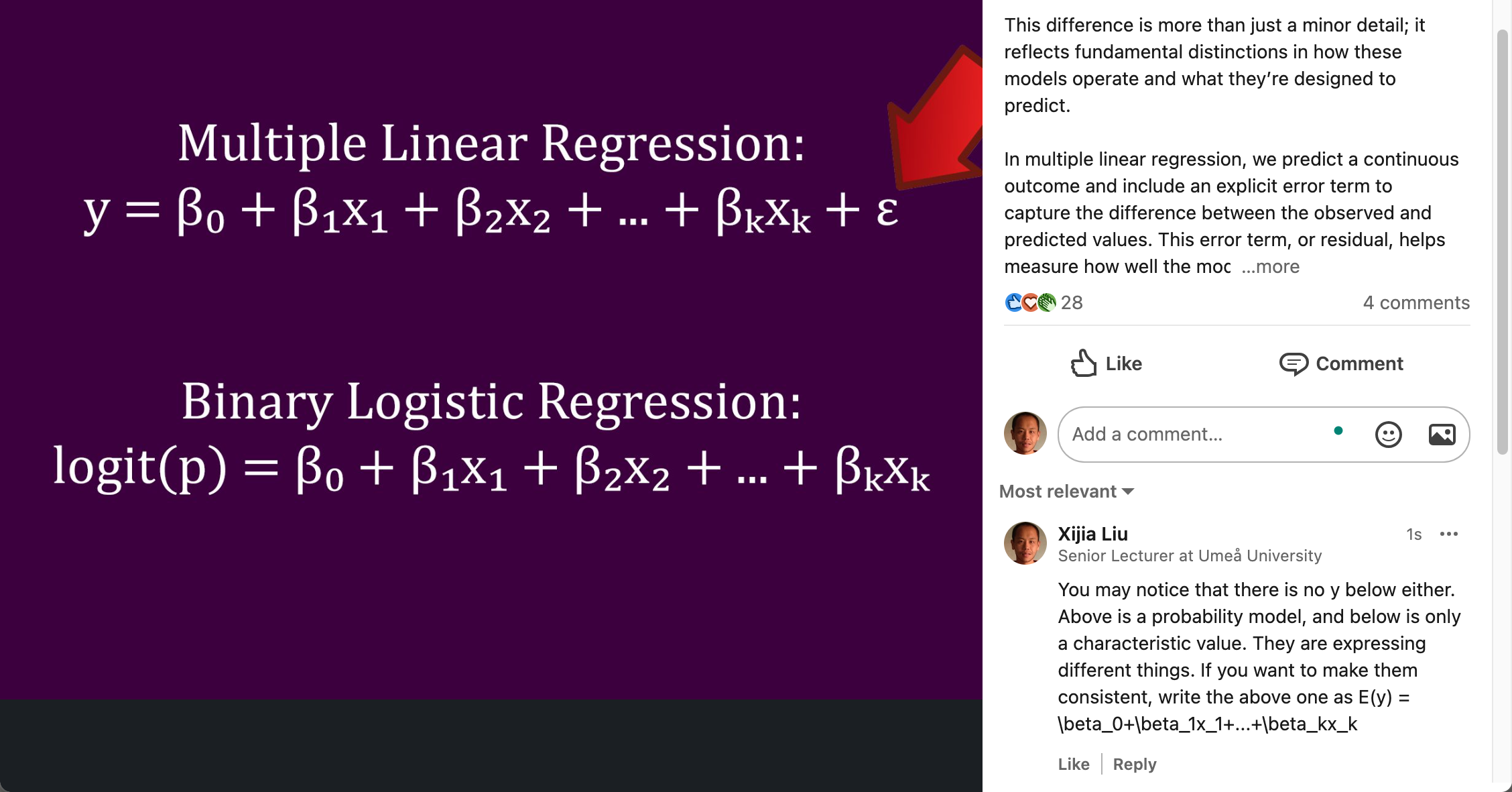
Let’s go back to our previous discussion: what is the main issue with using linear regression models for classification problems? First, we need to clarify one point: what is the essence of the linear regression model? Recall the discussion of maximum likelihood estimation of linear regression model. The essence of the linear regression model is to predict the expected value of the target variable using a linear combination of the feature variables, i.e. \[ \text{E}(y | \textbf{x}) = w_0 + w_1x_1 + w_2x_2 + \dots + w_px_p \] This is quite normal for a continuous target variable. However, when we try to extend this model to classification problems, we encounter new issues.
Essentially, we are trying to model the expected value of target variable as the weighted sum of feature variables, when we apply linear regression model to a classification problem. However, in classification problems, the target variable is a categorical variable. For categorical variables, the assumption of a normal distribution is completely unreasonable. We need to use discrete distributions to characterize the distribution of these variables, for example, using binary distribution for a binary classification problem, i.e. \(y \sim \text{Ber}(\pi)\), \[ y = \left\{ \begin{matrix} 1 & \text{Positive case} \\ 0 & \text{Negative case} \end{matrix} \right. \] What is the expected value of a binary distributed random variable? It is the probability of \(y = 1\), i.e. \(\text{E}(y) = \pi\). So, we are using the following equation \[ \pi|\textbf{x} = \text{E}(y|\textbf{x}) = w_0 + w_1x_1 + w_2x_2 + \dots + w_px_p \] If we analyze the range of values on both sides of the equation, it is not difficult to identify the critical flaw in using linear regression to handle classification problems. The left side of the equation represents a probability value, with a range of \([0, 1]\), while the right side can take any real number. Clearly, fitting a probability with an arbitrary real number is unreasonable and this is where the problem lies.
2.2 Model Construction
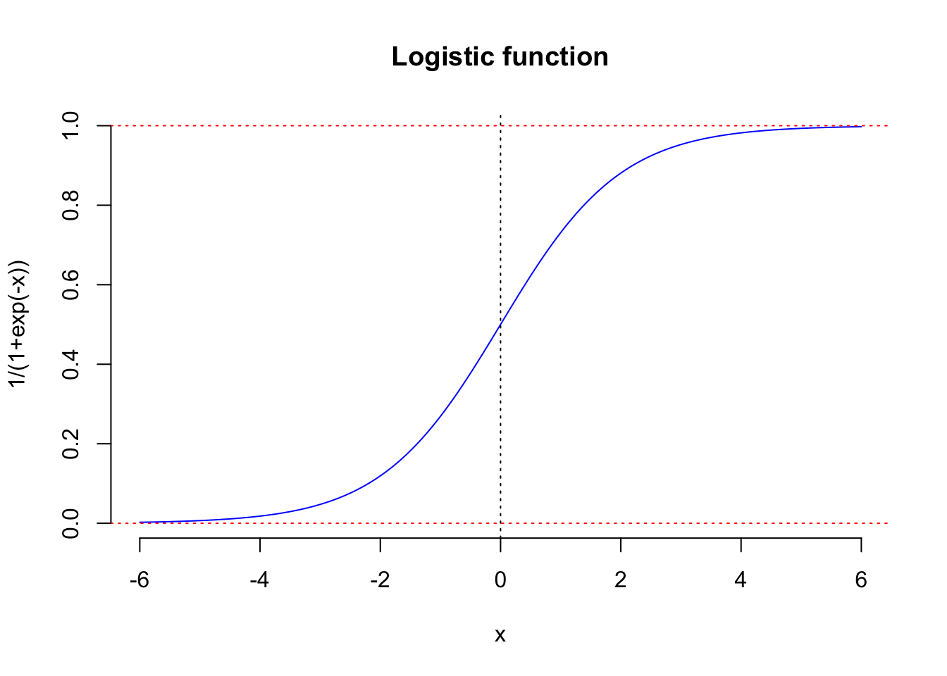
To address the issue mentioned above, mathematicians proposed an idea: using a function to transform values that span the entire real number axis into a fraction. This transformation function is the well-known logistic function, \[ \phi(t) = \frac{1}{1+e^{-t}} \] The graph of the logistic function is shown in the figure below. We can see that through its transformation, the output for any input \(x\) lies between the two red dashed lines, meaning it is a fraction.
With the help of the logistic function, we can start building our logistic regression model.
For a binary classification problem, we assume that the target variable follows a binary distribution, where the probability of a positive case is calculated as the logistic transformed weighted sum of the feature variables plus a constant. In a formal mathematical language, logistic regression model presents a probability model, \(y\sim \text{Ber}\left( \pi(\textbf{x}; \textbf{w}) \right)\), where \[ \pi(\textbf{x}; \textbf{w}) = \phi(w_0 + w_1x_1 + w_2x_2 + \dots + w_px_p) = \frac{1}{1 + e^{-(w_0 + w_1x_1 + w_2x_2 + \dots + w_px_p)}} \] As can be seen from the above model, the logistic regression model essentially provides us with a mechanism for calculating the posterior probability of the target variable, i.e. \[ \Pr\left( Y = 1 | \textbf{x} \right) = \frac{1}{1 + e^{-(w_0 + w_1x_1 + w_2x_2 + \dots + w_px_p)}} \] In other words, once we have obtained all the parameters \(\textbf{w}\), we can evaluate the posterior probability using the values of the feature variables. If you still remember the classification rule of the GDA classifier, \[ \widehat{y} = \arg \max_{y} \Pr(y| \textbf{x}) \] then it is natural that the logistic regression model can be used as a classifier. Simply speaking, if the posterior probability evaluated by logistic regression, \(\Pr\left( Y = 1 | \textbf{x}_{new} \right) > 0.5\), then we should classify this new case as positive, otherwise, negative group.
2.3 Logistic Regression in R
In R, we can apply glm function to estimate logistic regression model, and the usage is very simple.
# usage of function `glm` for estiamte logistic regression
model = glm(MODEL_EXPRESSION, family = binomial(), DATA)
Similar to using lm to estimate linear regression, we first need to specify the model expression, and the rules are the same. However, the difference is that we need to verify another argument, family, as Binomial. This argument mainly determines the type of the target variable \(y\), that is, it specifies its distribution. “Binomial” means that the target variable follows a binomial distribution, which implies that \(y\) has a binary distribution. More demonstration by examples will be presented in the next subsection.
Quiz: Can you guess what kind of model will be returned if you specify family as gaussian?
2.4 Decision Boundary
In the field of statistics, logistic regression is typically considered a type of generalized linear regression model. Generalized linear models (GLMs) form a large family of models, which includes common distributions for the response variable, such as Poisson regression, multinomial regression, beta regression, and so on. Logistic regression is also often referred to as a nonlinear regression model because, in the end, it projects the feature variables onto a nonlinear surface, as shown in the figure below.
LHS: Multivariate linear regression model. RHS: Logistic regression model, the surface is \(\phi(w_0 + w_1X_1+ w_2X2)\), where \(\phi\) is the logistic function.
Question: If logistic regression is considered a nonlinear statistical model, is it a nonlinear classifier?
R example:
Let’s address the previous example with outliers. To solve this problem, we can kill three birds with one stone: learn an R example, validate the robustness of logistic regression, and finally, experimentally obtain the answer to the above question. The data set can be downloaded here.
I show you the dataset for the problem we discussed before and visualize it in a scatter plot.
head(dat) x1 x2 y
1 1.419 2.280 1
2 0.553 3.838 1
3 1.704 2.422 1
4 1.331 3.096 1
5 1.660 1.397 1
6 2.434 1.712 1color_obs = ifelse(dat$y==1, "blue", "red")
par(mar = rep(1,4))
plot(dat$x1, dat$x2, col = color_obs, pch = 20,
cex = 2, axes = F, xlab="", ylab = "")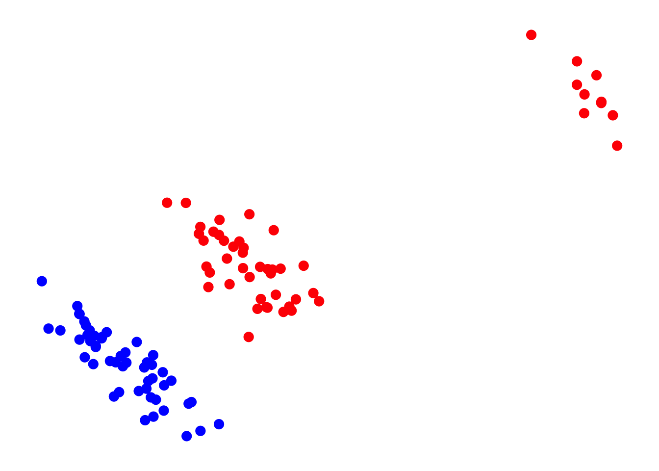
Let’s first demonstrate how to obtain the classification boundary for the linear regression model. By the way, the answer to the previous quiz is the linear regression model. That is, if we set the family argument to Gaussian, we will get a linear regression model. In other words, its output is the same as the output from the lm function. Now, let’s use it to calculate the model parameters.
m_linReg = glm(y~., data = dat, family = "gaussian")
summary(m_linReg)
Call:
glm(formula = y ~ ., family = "gaussian", data = dat)

Coefficients:
            Estimate Std. Error t value Pr(>|t|)
(Intercept)  1.08317    0.06386  16.962  < 2e-16 ***
x1          -0.03156    0.01510  -2.091   0.0392 *
x2          -0.10966    0.02241  -4.894 3.94e-06 ***
---
Signif. codes:  0 '***' 0.001 '**' 0.01 '*' 0.05 '.' 0.1 ' ' 1

(Dispersion parameter for gaussian family taken to be 0.1108737)

    Null deviance: 25.000  on 99  degrees of freedom
Residual deviance: 10.755  on 97  degrees of freedom
AIC: 68.805

Number of Fisher Scoring iterations: 2
Next, let’s render the classification boundary of the classifier based on this model. Similar to how we rendered the classification boundary for k-NN previously, we will first generate a grid for the 2D feature space. Then, we will use our model to classify each grid point and present the decision boundary.
x1 = seq(-1,16,0.1)
x2 = seq(0,14,0.1)
d = expand.grid(x1 = x1, x2 = x2)
class(d)
[1] "data.frame"scores = predict(m_linReg, d)
color_test = ifelse(scores > 0.5, "#D6E8FF", "#FFD6D6")par(mar = rep(1,4))
plot(dat$x1, dat$x2, col = color_obs, pch = 20,
cex = 2, axes = F, xlab="", ylab = "")
points(d$x1, d$x2, col = color_test, pch = 20, cex = 0.5)
points(dat$x1, dat$x2, col = color_obs, pch = 20, cex = 2)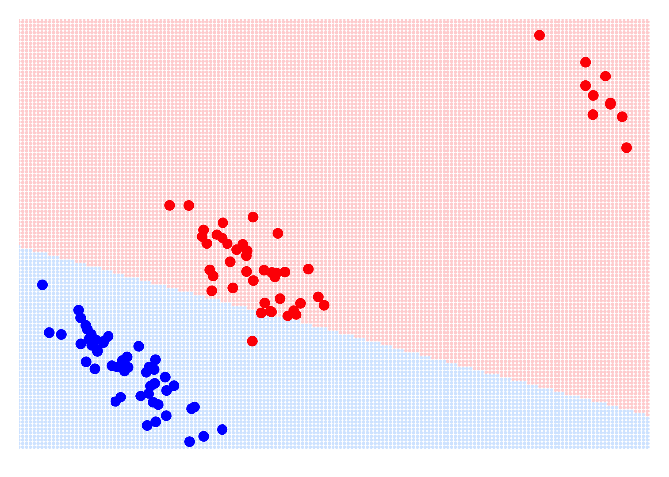
As we observed earlier, the classifier based on the linear regression model is very sensitive to outliers. Even in such a simple classification problem, it makes errors in certain areas. Now, let’s take a look at the performance of the classifier based on the logistic regression model.
m_LogReg = glm(y~., data = dat, family = binomial())res_pred = predict(m_LogReg, d, type = "response")
range(res_pred)[1] 2.220446e-16 1.000000e+00Here, we use the predict function to predict the label for each grid point. Note that in the function above, we set the type argument to ‘response’, so we will obtain the posterior probability for each grid point based on its coordinates. Then, we can classify the points using the standard cutoff of 0.5. Finally, we use this grid to present the classification boundary of the classifier based on the logistic regression model.
color_test = ifelse(res_pred > 0.5, "#D6E8FF", "#FFD6D6")par(mar = rep(1,4))
plot(dat$x1, dat$x2, col = color_obs, pch = 20,
cex = 2, axes = F, xlab="", ylab = "")
points(d$x1, d$x2, col = color_test, pch = 20, cex = 0.5)
points(dat$x1, dat$x2, col = color_obs, pch = 20, cex = 2)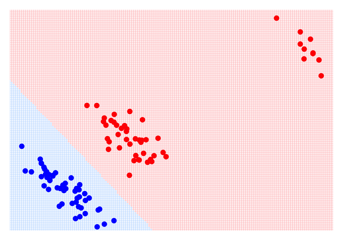
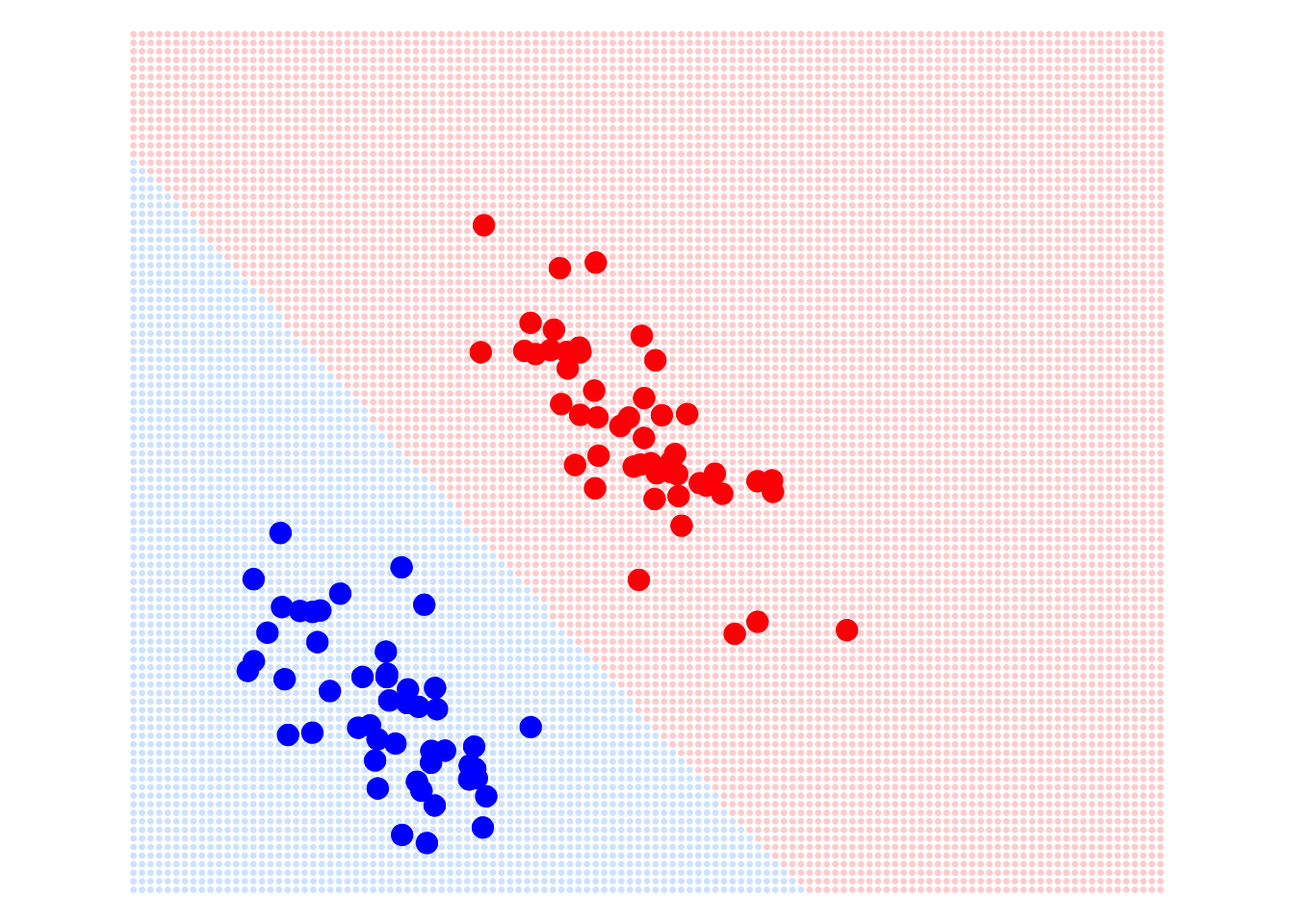
As we can see, using logistic regression as a classifier allows us to correct the impact of outliers. Additionally, we can observe that the classification boundary of the logistic regression classifier is also a straight line, meaning it is a linear classifier. In fact, this conclusion is not difficult to reach. From the principle of the classifier, the classification boundary of the logistic regression classifier is: \[ \Pr(Y = 1|\textbf{x}) = \phi(\text{scores}) = \frac{1}{1 + e^{-(w_0 + w_1X_1 + \dots + w_pX_p)}} = \frac{1}{2} \] If we simplify this formula, we can derive the classification boundary of the logistic regression classifier \[ w_0 + w_1X_1 + \dots + w_pX_p = 0 \] So, the classifier based on logistic regression is a linear classifier.
3. Cross-Entropy Loss and Penalized Logistic Regression
3.1 Cross-entropy Loss and Likelihood function
Above, we conceptually explained the logistic regression model and its classifier and demonstrated its implementation in R. Next, we will address a more theoretical question: how to train our model, or in other words, how to estimate the model parameters. This question can be approached from both machine learning and statistical modeling perspectives, yielding consistent conclusions.
Strategy: From the machine learning perspective, it is relatively easy to formulate the optimization problem for the logistic regression model. However, different from MSE loss, to fully understand the cross-entropy loss function, we would need to learn some additional concepts from information theory. Since we have already studied likelihood theory, deriving the objective function (i.e., the likelihood function) from this perspective is comparatively straightforward. Therefore, to simplify the learning process, I will introduce the cross-entropy loss from the machine learning perspective and then interpret it through the lens of likelihood theory. In the near future, you can revisit this concept from the information theory perspective when you study neural networks.
3.1.1 Cross-entropy Loss
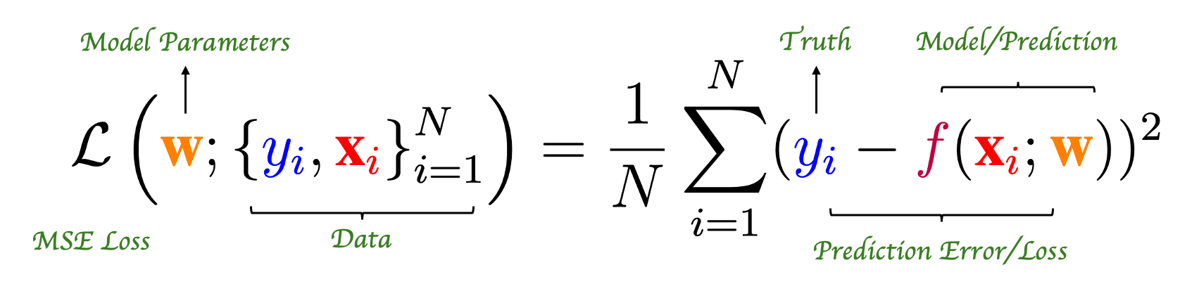
Let us recall the brute-force method we used when training a regression model. First, we define a loss function, specifically the MSE loss, which we use to evaluate the model’s performance.
After defining the loss function, we can select the optimal model based on the performance corresponding to different sets of model parameters. In the absence of an efficient algorithm, brute-force computation is the simplest solution. However, for a well-defined optimization problem, smart mathematicians would never resort to brute-force computation so easily. This has led to the development of various algorithms for training models, e.g. gradient descent algorithm.
Alright, let’s return to the logistic regression model. How do we determine its model parameters? Similarly, we can design a loss function for the model and formulate it as an optimization problem. However, for a classification problem, we cannot directly calculate the model error and take the average, as we do in regression problems. Instead, the most commonly used loss function for classification problems is the cross-entropy loss: \[ \mathcal{L}\left(\textbf{w};\left\{ y_i, \textbf{x}_i \right\}_{i=1}^N \right) = -\frac{1}{N}\sum_{i = 1}^N \left\{ y_i\log( \pi(\textbf{x}_i, \textbf{w}) ) + (1-y_i)\log(1-\pi(\textbf{x}_i, \textbf{w})) \right\} \] Similar to training regression problems, the model parameters of logistic regression can be obtained by optimizing the cross-entropy loss, i.e., \[ \hat{\textbf{w}} = \arg\max_{\textbf{w}} \mathcal{L}(\textbf{w};\left\{ y_i, \textbf{x}_i \right\}_{i=1}^N) \]
Note: The cross-entropy loss is undeniably famous. You will encounter it again when you study neural network models and deep learning in the future.
Unlike regression problems, optimizing the cross-entropy loss does not have an analytical solution. This means that we must use numerical algorithms to find the optimal solution. Typically, we use second-order optimization algorithms to estimate the parameters of logistic regression, such as the Newton-Raphson algorithm you practiced in Lab 1. In broader fields, like optimizing deep neural network models, the gradient descent algorithm is commonly used. We will only touch on this briefly here, and I will discuss it in more detail in the future.
Think: Why can’t we design the loss function using prediction error like in regression problems? What would happen if we did?
3.1.2 Maximum Likelihood Estimation
Cross-entropy loss is not as easy to understand as MSE loss; you need to learn some information theory to fully grasp it. But don’t worry, here we will approach it from the perspective of statistical theory, specifically from the concept of maximum likelihood estimation (MLE), which you have already studied. In the end, you will find that the likelihood function of MLE and the cross-entropy loss are equivalent.
Suppose we have a set of training observations, \(\left\{ y_i, \textbf{x}_i \right\}_{i = 1}^N\). The distribution of the target variable is Binary distribution, i.e. \[ \Pr\left( y_i, \pi(\textbf{x}_i, \textbf{w}) \right) = \pi(\textbf{x}_i, \textbf{w}) ^{y_i} (1-\pi(\textbf{x}_i, \textbf{w}))^{1 - y_i} \] where \(y_i = 1 \text{ or } 0\). Since we have independent observations, the joint likelihood of the training sample is \[ L\left(\textbf{w}; ;\left\{ y_i, \textbf{x}_i \right\}_{i=1}^N \right) = \prod_{i = 1}^{n} \pi(\textbf{x}_i, \textbf{w}) ^{y_i} (1-\pi(\textbf{x}_i, \textbf{w}))^{1 - y_i} \] The log-likelihood function is \[ \ell\left(\textbf{w}; \left\{ y_i, \textbf{x}_i \right\}_{i=1}^N\right) = \sum_{i = 1}^N \left\{ y_i\log( \pi(\textbf{x}_i, \textbf{w}) ) + (1-y_i)\log(1-\pi(\textbf{x}_i, \textbf{w})) \right\} \] The MLE of \(\textbf{w}\) is \[ \hat{\textbf{w}}_{\text{MLE}} = \arg\max_{\textbf{w}} \ell\left(\textbf{w};\left\{ y_i, \textbf{x}_i \right\}_{i=1}^N\right) \]
Now we can compare the likelihood function and the cross-entropy loss function. Upon comparison, you will find that they differ only by a negative sign. Therefore, maximizing the likelihood function is equivalent to minimizing the loss function; they are interchangeable. So, if you want to understand cross-entropy loss, start by approaching it from the perspective of likelihood analysis.
3.2 Penalized Logistic Regression
In the previous lecture, we discussed the shrinkage and sparse versions of the regression model. Through these, we can both avoid the risk of overfitting and indirectly obtain feature selection results. For classification problems, we have similar tools available, that is penalized logistic regression.
Let’s first recall the idea of penalized regression. We define a set of candidate models by adding the calculation of the budget for the model parameter values, i.e., \[ \textcolor[rgb]{1.00,0.00,0.00}{\text{Candidate Models}} = \textcolor[rgb]{1.00,0.50,0.00}{\text{Full Model}} + \textbf{Budget}(\textbf{w}). \] With the general form of all candidate models, the penalized regression problem can be formulated as \[ \min_{\textbf{w}} \left\{ \mathcal{L}_{mse}\left( \textbf{w}; \left\{ y_i, \textbf{x}_i \right\}_{i=1}^N \right) + \lambda\textbf{Budget}(\textbf{w}) \right\} \] where the mse loss is just the sum squared residuals, and the budget term can be \(L_1\) norm, i.e. LASSO, or \(L_2\) norm, i.e. ridge regression.
Now, let’s return to the logistic regression model. The clever among you might have already realized that the difference between penalized logistic regression and the previous penalized regression is simply the choice of the loss function. If we replace the MSE loss in the above formula with the cross-entropy loss, we obtain the optimization problem for penalized logistic regression, and the optimal solution is the penalized logistic regression model parameters.
Similarly, if we choose the \(L_2\) norm, we will get a shrinkage solution, whereas the \(L_1\) norm will provide us with a sparse solution and serve as an important tool for feature selection in classification problems. In addition, we will encounter many variations of penalty terms, such as the Elastic net penalty, \[ \alpha \times \sum_{j = 1}^p |w_j| + (1- \alpha) \times \sum_{j = 1}^p w_j^2 \] where \(\alpha\) is an extra hyper-parameter taking value in \([0,1]\). From the above formula, it is easy to see that the calculation of the parameter value budget in elastic net is intermediate between ridge regression and LASSO. If the parameter \(\alpha\) is set to 1, the elastic net degenerates into the LASSO penalty. Conversely, if \(\alpha\) is set to 0, we get the \(L_2\) penalty, which corresponds to ridge regression. When \(\alpha\) takes any value between 0 and 1, we obtain the elastic net. In other words, the elastic net is a convex combination of the \(L_1\) penalty and the \(L_2\) penalty. This setup makes the corresponding candidate models more flexible. Of course, the trade-off is that we need to consider an additional hyperparameter. Alright, let’s stop here for now. We will explain the implementation of penalized logistic regression in more detail in the upcoming labs.
Course Conclusion
Alright, we can finally take a break. In this course, we have introduced some important concepts of machine learning through simple models. I hope the gap between basic statistics and basic machine learning isn’t too wide. I also hope that you will revisit and digest these materials, laying a solid foundation for further learning in machine learning. Thank you for your attention, and I look forward to meeting you again here in the near future.
Wishing you all the best!
Xijia Liu
December 6, 2024, Umeå