Solutions to Exercises in Lab 4

we implement and practice k-nearest neighbors method and subset selection methods with Breast cancer data and simulated data.

Task 1: About KNN and Cross Validation

In this task, we apply K-nearest neighbor method to Breast cancer data. We use variables radius, texture and smoothness to predict the target variable diagnosis.

Import data

# Import data
dat_tr = read.table("BreastCancerTrain.txt", header = T, sep = ",")
dat_te = read.table("BreastCancerTest.txt", header = T, sep = ",")
dat_tr = dat_tr[,c(1,2,3,6)]
dat_te = dat_te[,c(1,2,3,6)]

Task 1.1: Practice KNN method

Read the help document of the function knn in library class first. This exercise aims to analyze how the choice of \(k\) affects the KNN method’s performance on training and test datasets and identify any patterns in overfitting or underfitting as \(k\) varies. Follow the instructions below to complete your experiment, and then draw your conclusions based on the experimental results.

Solutions:

Step 1:

K = seq(1,300,2)
num_k = length(K)
res_tr = res_te = numeric(num_k)

Step 2:

library(class)
for(i in 1:num_k){
  y_tr_pre = knn(dat_tr[,-1], dat_tr[,-1], dat_tr[,1], K[i])
  res_tr[i] = mean(y_tr_pre == dat_tr[,1])
  y_te_pre = knn(dat_tr[,-1], dat_te[,-1], dat_tr[,1], K[i])
  res_te[i] =mean(y_te_pre == dat_te[,1])  
}

Step 3:

plot(1:num_k, res_tr, type = "b", col = "red", pch = 20, cex = 0.5,
     ylab = "Accuracy", xlab = "k", ylim = range(c(res_tr, res_te)))
points(1:num_k, res_te, type = "b", col = "blue", pch = 20, cex = 0.5)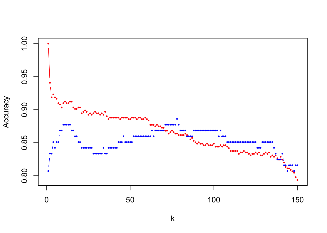

Task 1.2: Practice LOOCV

Read the help document of the function knn.cv in library class first. Apply LOOCV to select the best hyper-parameter \(k\) and test the model performance in the testing set.

Tips: You can apply function knn.cv to perform LOOCV to select the best hyper-parameter. The suggested instruction:

Step 1:

# define all the candidate values
K = seq(1,300,2)
num_k = length(K)
# creat a vector 'cv_acc' to save all the cross validation results for all candidate models
cv_acc = numeric(num_k)

Step 2:

for(i in 1:num_k){
  # loop over all candidate models
  y_pre = knn.cv(train = dat_tr[,-1], cl = dat_tr[,1], k = K[i]) # get the prediction by leave one out cross validation
  cv_acc[i] = mean(dat_tr[,1] == y_pre) # calculate the cv accuracy for the ith candidate model
}
plot(1:num_k, cv_acc, type="b", pch = 20, cex = 0.5, xlab = "k")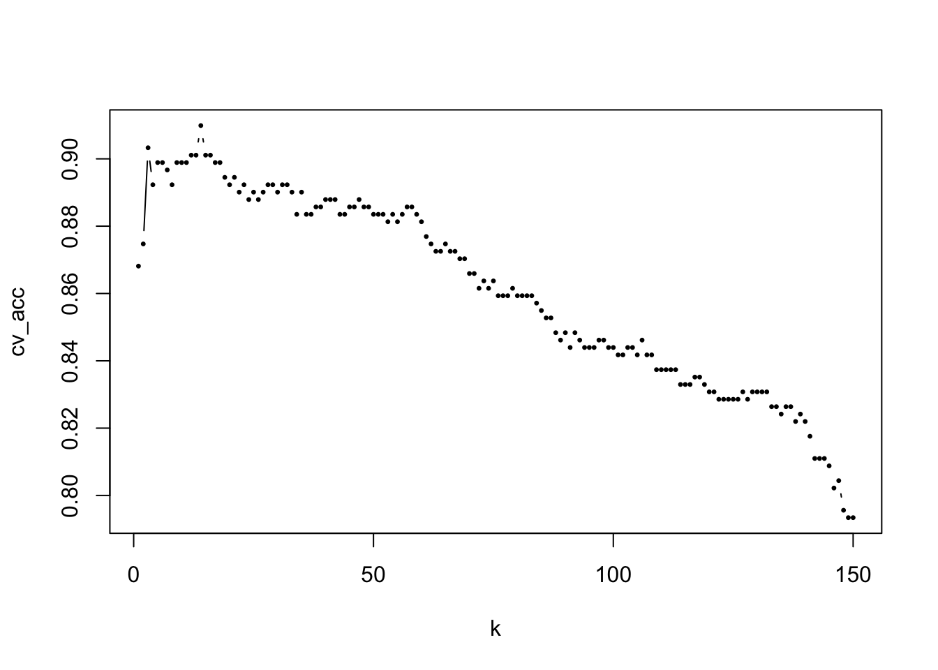

Step 3:

opt_k = which(cv_acc==max(cv_acc)) # find the optimal K
K[opt_k]

[1] 27

# Estimate the model performance with testing data
y_pre = knn(train = dat_tr[,-1], test = dat_te[,-1], cl = dat_tr[,1], k = K[opt_k])
mean(dat_te[,1] == y_pre)

[1] 0.877193

Task 1.3: Practice 5-fold Cross Validation

Tune the hyper-parameter by 5-fold cross validation. Estimate the model performance of the optimal model with testing set.

Note: Function knn.cv only provide LOOCV option. So, you need to implement the 5-fold CV by your own code.

Solutions:

K = seq(1,300,2)
num_k = length(K)
set.seed(8312)
cv_k_acc = numeric(num_k)
ID = matrix(sample(1:445), nrow = 5) # randomly split the sample into k folds
# each row of 'ID' contains all the id of observations in the corresponding fold

Solutions: Since each row in ID contains the index of one fold, we can write a for loop to implement 5-fold validation.

for(i in 1:num_k){
  temp_res = numeric(5)
  for(j in 1:5){
    y_pre = knn(train = dat_tr[-ID[j,],-1], # pick up the feature variables of observations not in the jth fold
                test = dat_tr[ID[j,],-1], # predict on the observations in the jth fold
                cl = dat_tr[-ID[j,],1], # target variable of observations not in the jth fold
                k = K[i])
    temp_res[j] = mean(y_pre == dat_tr[ID[j,],1]) # accuracy of the current model for the jth fold
  }
  cv_k_acc[i] = mean(temp_res) # overall cv accuracy for the jth fold
}
plot(1:num_k, cv_k_acc, type="b", pch = 20, cex = 0.5)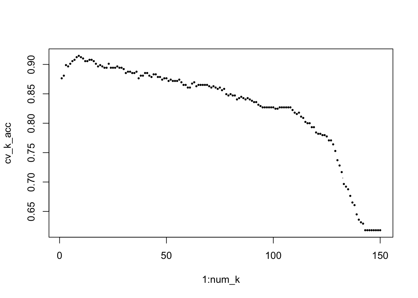

Solutions: Find the optimal model selected by 5-fold CV and estimate the model performance.

opt_k = which(cv_k_acc==max(cv_k_acc)) # find the optimal K
K[opt_k]

[1] 17

# Estimate the model performance with testing data
y_pre = knn(train = dat_tr[,-1], test = dat_te[,-1], cl = dat_tr[,1], k = K[opt_k])
mean(dat_te[,1] == y_pre)

[1] 0.8684211

Task 2: About Feature Selection

In this task, we will use simulated data to practice feature selection methods. The simulated data can be generated using the following R code. From the code, we can see that the target variable is primarily determined by the first five feature variables. Below, we randomly display the first six observations of five feature variables and the target variable \(y\).

set.seed(8312)
n = 500
p = 20 
X = matrix(rnorm(n * p), nrow = n, ncol = p)
w = c(2, -3, 1, 2.3, 1.5, rep(0, p-5))
y = X %*% w + rnorm(n, mean = 0, sd = 1)
dat = data.frame(X, y = y)
rm( X, w, y)
head(dat[, c(sort(sample(1:20, 5)), 21)])

          X7          X8         X13         X14        X18         y
1 -0.4051647  0.04860872  0.03389675 -2.51265909 -0.7737131  2.683957
2 -0.3300477 -1.19580506 -1.48307329 -0.24639241 -0.7631660 -2.255025
3  0.8251963  0.33617031 -0.22148474  0.27703785 -0.4178979 -7.106195
4 -0.8314352  1.32395677  1.20709742  1.84552276 -0.8829887  2.433349
5 -0.5919659 -0.06201140  0.15292587  0.28684091 -1.6195710 -1.023411
6 -2.0953279 -1.45533806 -0.50448883  0.06009562  0.4953250 -2.891946

Task 2.1: Practive `leaps` package

Read the help document of function regsubsets. Apply this function to do best subset selection on the simulated data, dat. Print out the names of variable selected in the candidate model with 8 feature variables and their model coefficients.

Tips: Two options to get the regression coefficients:

You can find the included variables of the candidate model with 8 feature variables by the following code.

summary(m)$which # m: the output of `regsubsets`

Use function coef to extract the selected variables. You need to specify two arguments, the output of regsubsets function and the id of target candidate model.

library(leaps)
m1 = regsubsets(y~., dat, nvmax = 10) # if you want to do forward/backward selection, then you need to add 'method' in the function
# summary(m1)

summary(m1)$which

   (Intercept)    X1   X2    X3    X4    X5    X6    X7    X8    X9   X10   X11
1         TRUE FALSE TRUE FALSE FALSE FALSE FALSE FALSE FALSE FALSE FALSE FALSE
2         TRUE FALSE TRUE FALSE  TRUE FALSE FALSE FALSE FALSE FALSE FALSE FALSE
3         TRUE  TRUE TRUE FALSE  TRUE FALSE FALSE FALSE FALSE FALSE FALSE FALSE
4         TRUE  TRUE TRUE FALSE  TRUE  TRUE FALSE FALSE FALSE FALSE FALSE FALSE
5         TRUE  TRUE TRUE  TRUE  TRUE  TRUE FALSE FALSE FALSE FALSE FALSE FALSE
6         TRUE  TRUE TRUE  TRUE  TRUE  TRUE FALSE FALSE FALSE FALSE FALSE FALSE
7         TRUE  TRUE TRUE  TRUE  TRUE  TRUE FALSE FALSE FALSE FALSE FALSE FALSE
8         TRUE  TRUE TRUE  TRUE  TRUE  TRUE FALSE FALSE FALSE FALSE FALSE FALSE
9         TRUE  TRUE TRUE  TRUE  TRUE  TRUE FALSE FALSE FALSE FALSE FALSE FALSE
10        TRUE  TRUE TRUE  TRUE  TRUE  TRUE  TRUE FALSE FALSE FALSE FALSE FALSE
     X12   X13   X14   X15   X16   X17   X18   X19   X20
1  FALSE FALSE FALSE FALSE FALSE FALSE FALSE FALSE FALSE
2  FALSE FALSE FALSE FALSE FALSE FALSE FALSE FALSE FALSE
3  FALSE FALSE FALSE FALSE FALSE FALSE FALSE FALSE FALSE
4  FALSE FALSE FALSE FALSE FALSE FALSE FALSE FALSE FALSE
5  FALSE FALSE FALSE FALSE FALSE FALSE FALSE FALSE FALSE
6  FALSE FALSE FALSE FALSE FALSE FALSE  TRUE FALSE FALSE
7   TRUE FALSE FALSE FALSE FALSE FALSE  TRUE FALSE FALSE
8   TRUE FALSE FALSE FALSE FALSE FALSE  TRUE  TRUE FALSE
9   TRUE FALSE FALSE FALSE  TRUE FALSE  TRUE  TRUE FALSE
10  TRUE FALSE FALSE FALSE  TRUE FALSE  TRUE  TRUE FALSE

# solution 1
res = summary(m1)$which[8,-1]
temp_dat = dat[, res]
temp_dat$y = dat$y
m_temp = lm( y~., temp_dat )
m_temp$coefficients

(Intercept)          X1          X2          X3          X4          X5 
-0.04070300  1.98697488 -3.11149188  0.96235490  2.34621090  1.42697443 
        X12         X18         X19 
 0.06994639 -0.08102189  0.05768604

# solution 2
coef(m1, id=8) # find all the variables and coefficients in the optimal model with 8 features

(Intercept)          X1          X2          X3          X4          X5 
-0.04070300  1.98697488 -3.11149188  0.96235490  2.34621090  1.42697443 
        X12         X18         X19 
 0.06994639 -0.08102189  0.05768604

Task 2.2: Prediction with candidate models

Set random seed as 2024. Randomly split the data set into training and testing sets (80% VS 20%). Use the same method as task 2.1 to find all the candidate models. Apply the candidate model with 8 feature variables to the testing set and estimate the RMSE.

Tips: Function model.matrix can be used for preparing the data matrix for prediction, e.g.,

x_test = model.matrix(y~., dat_te)

set.seed(2024)
id = sample(1:dim(dat)[1], dim(dat)[1]*0.8)
dat_tr = dat[id,]
dat_te = dat[-id,]

m1 = regsubsets(y~., dat_tr, nvmax = 10)
x_test = model.matrix(y~., dat_te) # function for preparing prediction matrix for the testing set
coe = coef(m1, id = 7)
pred = x_test[, names(coe)]%*%coe # prediction. you also can implement this step by for loop
rmse = sqrt(mean((dat_te$y - pred)^2))
rmse

[1] 1.205906

Task 2.3: Select the final optimal model

With the same data spiting, find the optimal model by training-against-validation method. Estimate the model performance with the testing set.

id_train = sample(id, length(id)*0.8)
dat_training = dat_tr[id_train, ] 
dat_validating = dat_tr[-id_train, ] # further split training set as training and validation set

# find the best model 
m1 = regsubsets(y~., dat_training, nvmax = 10) 
x_val = model.matrix(y~., dat_validating)

res = numeric(10)
for(i in 1:10){
  coe = coef(m1, id = i)
  pred = x_val[, names(coe)]%*%coe
  res[i] = sqrt(mean((dat_validating$y - pred)^2))
}
plot(res)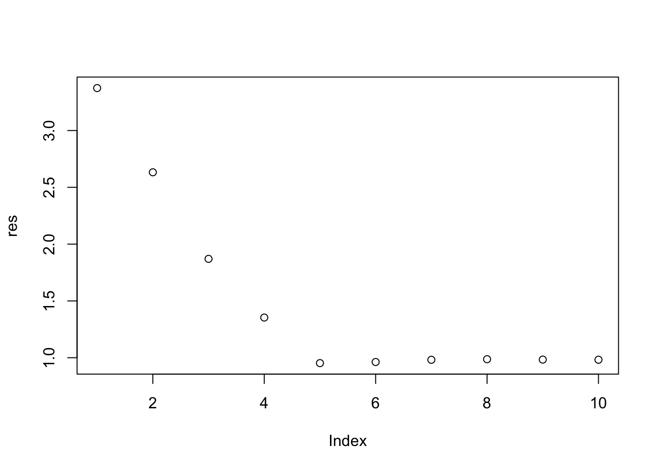

# we choose the model with 10 feature variables
# train the model with 10 feature variables and evaluate the model performance with the testing set.
opt = which(res == min(res))
opt

[1] 5

coef(m1, id = opt)

(Intercept)          X1          X2          X3          X4          X5 
-0.07504814  1.91831167 -3.13194720  0.92864807  2.31970426  1.44105002

res = summary(m1)$which[8,-1]
temp_dat = dat_tr[, res]
temp_dat$y = dat_tr$y

final_m = lm(y~., data = temp_dat)
pred = predict(final_m, dat_te)
mean((dat_te$y - pred)^2) # it the estimate model performance

[1] 1.433956

Task 2.4 (optinal): Practice `glmnet` package

Read the help document of cv.glmnet function in package glmnet first. Apply LASSO method to select the feature variables in dataset dat.

Note: If you are short on time, you can skip this task for now. We will focus on practicing this package in the lab next week.

Solutions:

library(glmnet)

Loading required package: Matrix

Loaded glmnet 4.1-8

set.seed(2024)
model = cv.glmnet( x = as.matrix(dat_tr[,-21]), y = dat_tr[,21],
                   nfolds = 10, alpha = 1, type.measure = "mse")
plot(model)

This figure illustrates the cross-validation results. The x-axis represents the logarithm of the penalty parameter, the y-axis shows the cross-validation MSE, and the top of the image indicates the number of variables included in the corresponding model. The first dashed line marks the model with the smallest cross-validation MSE, while the second dashed line indicates the model whose performance is within one standard deviation of the minimum MSE. In other words, the performance of the model marked by the second dashed line is very close to that of the model with the minimum MSE. However, in practice, we tend to prefer simpler models, which is why the model marked by the second dashed line is often selected.

model$lambda.min

[1] 0.03378175

model$lambda.1se

[1] 0.1363775

which(coef(model, s = "lambda.min")!=0)

 [1]  1  2  3  4  5  6  7  8  9 10 13 16 17 18 19 20

which(coef(model, s = "lambda.1se")!=0)

[1] 1 2 3 4 5 6

Above, the values of the penalty parameter and the corresponding indices of the selected variables for both the mse-min and mse-1se models are displayed.

Lecture 6 Homepage

Task 1: About KNN and Cross Validation

Task 1.1: Practice KNN method

Task 1.2: Practice LOOCV

Task 1.3: Practice 5-fold Cross Validation

Task 2: About Feature Selection

Task 2.1: Practive leaps package

Task 2.2: Prediction with candidate models

Task 2.3: Select the final optimal model

Task 2.4 (optinal): Practice glmnet package

Task 2.1: Practive `leaps` package

Task 2.4 (optinal): Practice `glmnet` package