1. Overfitting in Classification
In the previous section, we discussed the manifestations and consequences of the overfitting problem in regression. So, what about over fitting in classification problems? Let us first introduce a very intuitive classification algorithm, K Nearest Neighbors (KNN) method, and then use it to explore the over fitting issue in classification.
1.1 K Nearest Neighbors
The k-Nearest Neighbors (KNN) algorithm is a unique classifier that stands apart from linear classifiers. It’s based on one of the most intuitive ideas in machine learning: decisions are influenced by proximity. Unlike complex parametric methods, KNN operates in a way that mirrors human decision-making in everyday life.
Basic Idea: The fundamental concept of KNN can be likened to how we often follow trends or social cues. Imagine your neighbor buys a new type of lawn-mowing robot. Your spouse, noticing their satisfaction, might also want to buy one. KNN applies a similar principle in classification: it assigns a label to a data point based on the labels of its nearest neighbors in the feature space. This idea of “going with the flow” underpins the simplicity of KNN.
Algorithm: K-Nearest Neighbors Method
Inputs:
- \(\textbf{X}\), \(n\times p\) matrix, containing all \(p\) feature variables.
- \(y\), \(n \times 1\) array, the target variable.
- \(x_{new}\), \(p \times 1\) array, the feature values of a new observation.
- \(k\), the number of neighbors.
Steps:
- Calculate the distance between \(x_{new}\) and each sample points in \(\textbf{X}\).
- Find \(k\) sample points that have shortest distance to \(x_{new}\)
- Assign the label that is most common among the neighbors.
Output: The assigned label.
See the following demonstration. In this toy example, we have a binary classification problem with 2 feature variables. There are 10 observations in the training set. We apply 3-NN method to classify an arbitrary point in the 2D space according to the training samples.
Demo of KNN method
Formal formulation( NE ): KNN method can be easily generalized to multiple classification problems, \(M\) classes. For a multiple classification problem, suppose we have a training set \(\left\{\textbf{x}_i, y_i \right\}_{i = 1}^{N}\), where \(y_i\) takes value in a set of labels \(\left\{1, 2, \dots, M \right\}\). For a new observation point, \(\textbf{x}_{\text{new}}\), the posterior probability that the new point belongs to the \(j\)th class given the feature values can be evaluated as \[ \Pr(y=j|\textbf{x}_{\text{new}}) = \frac{1}{K}\sum_{i \in \mathbb{N}_k(\textbf{x}_{\text{new}})} \textbf{1}\{y_i = j\} \] where \(\mathbb{N}_k(\textbf{x}_{\text{new}})\) denotes the index set of k nearest neighbors of \(\textbf{x}_{\text{new}}\) in the training set, the indicator function \(\textbf{1}\{y_i = j\} = 1\) if \(y_i = j\) otherwise \(0\), and \(j = 1,2,\dots,M\). After evaluating the posterior probabilities, one can make the decision accordingly.
Discussion:
KNN method also can be applied to a regression problem. In a regression scenario, the prediction is the average value of the k nearest neighbor’s values of target variable. \[ y|\textbf{x}_{\text{new}} = \frac{1}{K}\sum_{i \in \mathbb{N}_k(\textbf{x}_{\text{new}})} y_i \]
KNN stands out as a special type of classifier for several reasons.
Memory-Based Model: KNN is often called a memory-based model because it requires storing all the training data. Without the training data, predictions cannot be made. This contrasts with classifiers like Gaussian Discriminant Analysis (GDA), where information from the training data is condensed into model parameters, eliminating the need to retain the original dataset. While many memory-based models exist, KNN is among the simplest.
Lazy Learner: Unlike most classifiers that estimate parameters during a training phase, KNN does not perform explicit training. Once the value of \(K\) is chosen, the algorithm simply relies on the stored data for prediction, making it a “lazy learner.”
Despite its simplicity, KNN is a powerful algorithm in many contexts, particularly when the dataset is small or when a straightforward decision boundary suffices.
1.2 Overfitting in Classification Problems
Obviously, the parameter \(K\) plays a critical role in KNN method. The number of neighbors we consider to make the final decision significantly impacts the model’s performance. Let’s look at the example below.
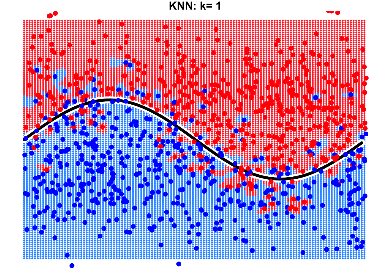
This is a binary classification problem where the true decision boundary is a sine curve. Due to the influence of noise variables, some observations cross the boundary. By using KNN with \(k=1\) and \(k=9\), we can observe the resulting decision boundaries as shown below.
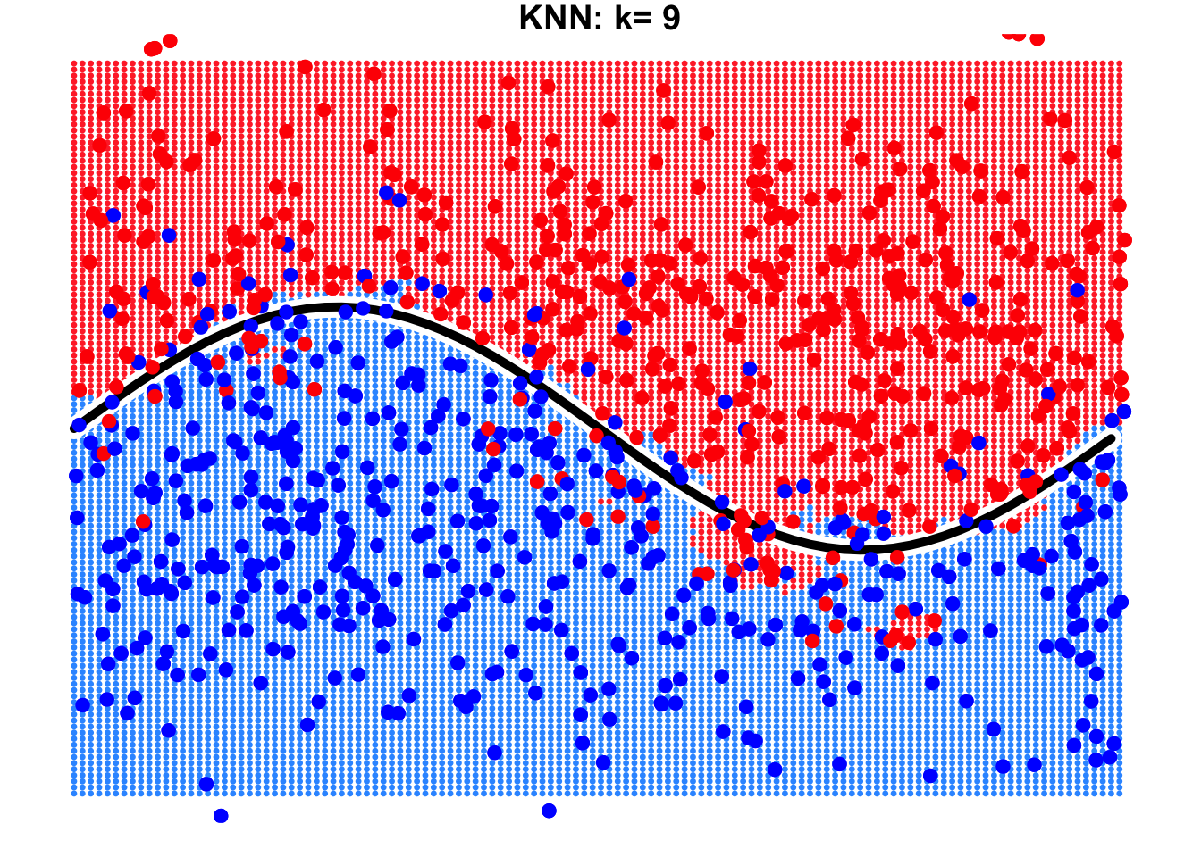
It is evident that the result with \(k=9\) is far better than that with \(k=1\). When \(k=9\), the true decision boundary of the sine curve can be largely identified or approximated by the KNN algorithm. However, when \(k=1\), we notice the emergence of many isolated “islands” on both sides of the true decision boundary. Errors occur in these “islands” because we focus excessively on individual observations in the training data, leading to overfitting.