Lecture 6: Model Validation and Selection

In this lecture, we focus on model validation and selection problem. Firstly, we will introduce KNN method and use it to interpret the over fitting problem in classification problems. At the same time, we also explained different types of parameters through the discussion of KNN, leading to the model selection problem. Then, we introduced various model validation methods. Finally, we discussed a specific model selection problem, namely feature selection. Here, we will introduce ridge regression and LASSO.

1. Overfitting in Classification

In the previous section, we discussed the manifestations and consequences of the overfitting problem in regression. So, what about over fitting in classification problems? Let us first introduce a very intuitive classification algorithm, K Nearest Neighbors (KNN) method, and then use it to explore the over fitting issue in classification.

1.1 K Nearest Neighbors

The k-Nearest Neighbors (KNN) algorithm is a unique classifier that stands apart from linear classifiers. It’s based on one of the most intuitive ideas in machine learning: decisions are influenced by proximity. Unlike complex parametric methods, KNN operates in a way that mirrors human decision-making in everyday life.

Basic Idea: The fundamental concept of KNN can be likened to how we often follow trends or social cues. Imagine your neighbor buys a new type of lawn-mowing robot. Your spouse, noticing their satisfaction, might also want to buy one. KNN applies a similar principle in classification: it assigns a label to a data point based on the labels of its nearest neighbors in the feature space. This idea of “going with the flow” underpins the simplicity of KNN.

Algorithm: K-Nearest Neighbors Method

Inputs:

\(\textbf{X}\), \(n\times p\) matrix, containing all \(p\) feature variables.
\(y\), \(n \times 1\) array, the target variable.
\(x_{new}\), \(p \times 1\) array, the feature values of a new observation.
\(k\), the number of neighbors.

Steps:

Calculate the distance between \(x_{new}\) and each sample points in \(\textbf{X}\).
Find \(k\) sample points that have shortest distance to \(x_{new}\)
Assign the label that is most common among the neighbors.

Output: The assigned label.

See the following demonstration. In this toy example, we have a binary classification problem with 2 feature variables. There are 10 observations in the training set. We apply 3-NN method to classify an arbitrary point in the 2D space according to the training samples.

Demo of KNN method

Formal formulation( NE ): KNN method can be easily generalized to multiple classification problems, \(M\) classes. For a multiple classification problem, suppose we have a training set \(\left\{\textbf{x}_i, y_i \right\}_{i = 1}^{N}\), where \(y_i\) takes value in a set of labels \(\left\{1, 2, \dots, M \right\}\). For a new observation point, \(\textbf{x}_{\text{new}}\), the posterior probability that the new point belongs to the \(j\)th class given the feature values can be evaluated as \[ \Pr(y=j|\textbf{x}_{\text{new}}) = \frac{1}{K}\sum_{i \in \mathbb{N}_k(\textbf{x}_{\text{new}})} \textbf{1}\{y_i = j\} \] where \(\mathbb{N}_k(\textbf{x}_{\text{new}})\) denotes the index set of k nearest neighbors of \(\textbf{x}_{\text{new}}\) in the training set, the indicator function \(\textbf{1}\{y_i = j\} = 1\) if \(y_i = j\) otherwise \(0\), and \(j = 1,2,\dots,M\). After evaluating the posterior probabilities, one can make the decision accordingly.

Discussion:

KNN method also can be applied to a regression problem. In a regression scenario, the prediction is the average value of the k nearest neighbor’s values of target variable. \[ y|\textbf{x}_{\text{new}} = \frac{1}{K}\sum_{i \in \mathbb{N}_k(\textbf{x}_{\text{new}})} y_i \]
KNN stands out as a special type of classifier for several reasons.
- Memory-Based Model: KNN is often called a memory-based model because it requires storing all the training data. Without the training data, predictions cannot be made. This contrasts with classifiers like Gaussian Discriminant Analysis (GDA), where information from the training data is condensed into model parameters, eliminating the need to retain the original dataset. While many memory-based models exist, KNN is among the simplest.
- Lazy Learner: Unlike most classifiers that estimate parameters during a training phase, KNN does not perform explicit training. Once the value of \(K\) is chosen, the algorithm simply relies on the stored data for prediction, making it a “lazy learner.”

Despite its simplicity, KNN is a powerful algorithm in many contexts, particularly when the dataset is small or when a straightforward decision boundary suffices.

1.2 Overfitting in Classification Problems

Obviously, the parameter \(K\) plays a critical role in KNN method. The number of neighbors we consider to make the final decision significantly impacts the model’s performance. Let’s look at the example below.

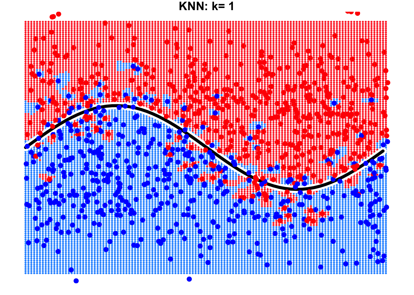
This is a binary classification problem where the true decision boundary is a sine curve. Due to the influence of noise variables, some observations cross the boundary. By using KNN with \(k=1\) and \(k=9\), we can observe the resulting decision boundaries as shown below.

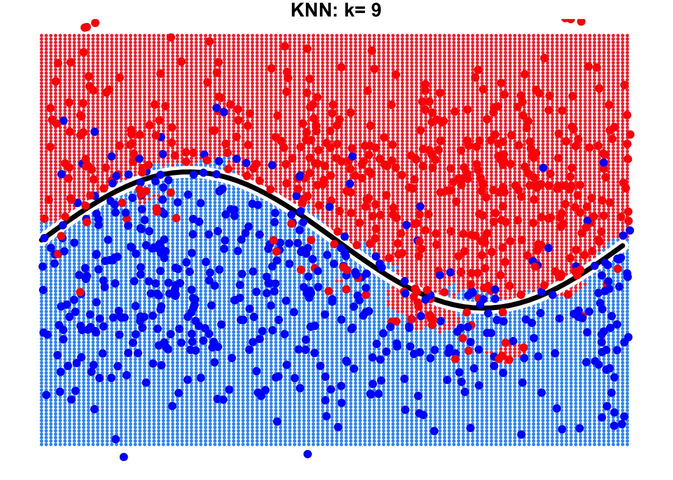
It is evident that the result with \(k=9\) is far better than that with \(k=1\). When \(k=9\), the true decision boundary of the sine curve can be largely identified or approximated by the KNN algorithm. However, when \(k=1\), we notice the emergence of many isolated “islands” on both sides of the true decision boundary. Errors occur in these “islands” because we focus excessively on individual observations in the training data, leading to overfitting.

2. Model Validation and Selection

2.1 Hyper-parameters

Think of a machine learning model like a car. Cars come in broad categories, such as SUVs, Hatchbacks, Sports cars, etc., each designed for a specific purpose. Within these categories, there are further variations, for instance, an SUV might be a compact crossover, a mid-size, or a full-size SUV, and the specific features like engine size or drivetrain vary between models.

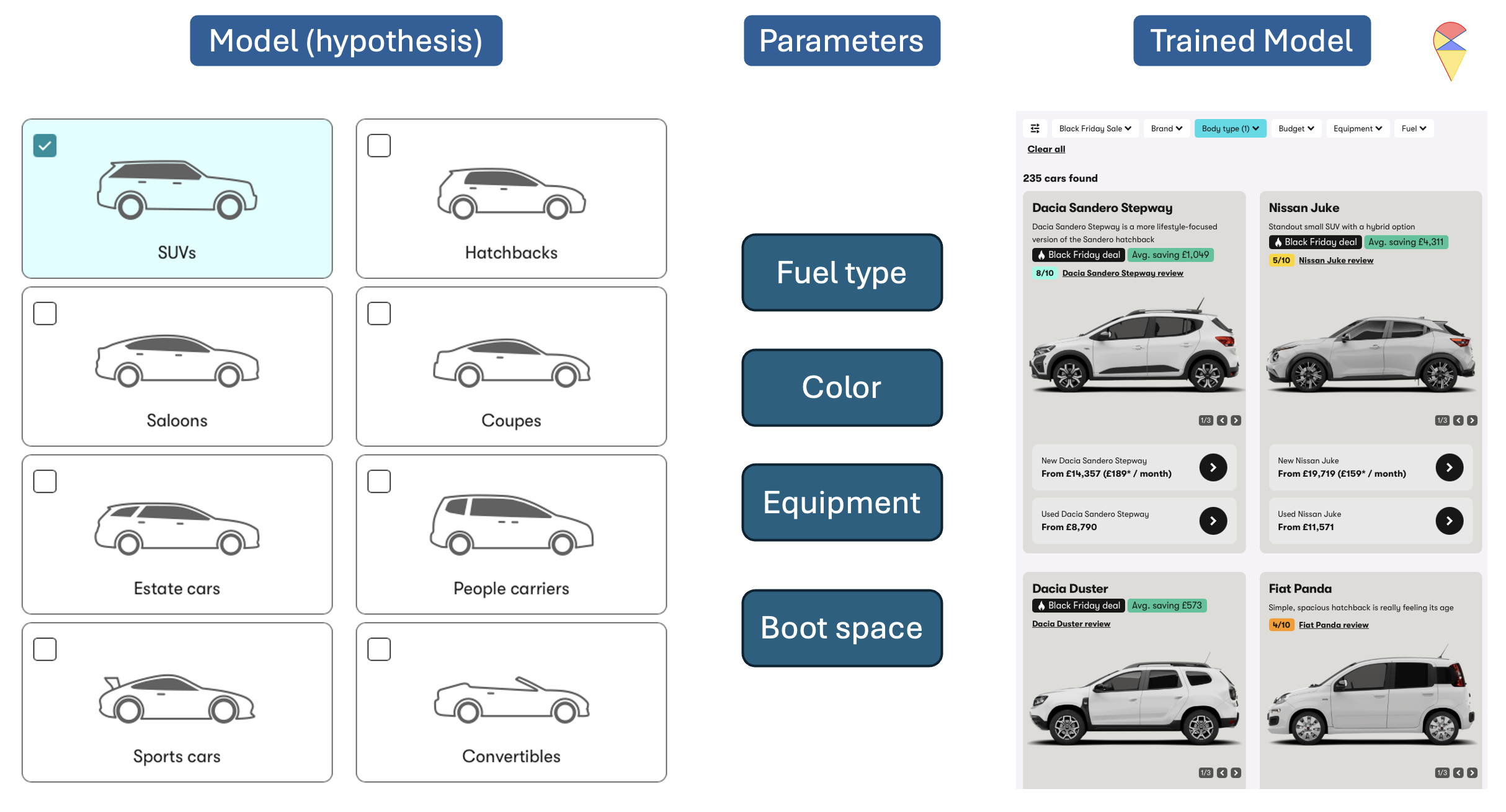
Have you ever bought a car? My experience was that I searched online and picked the cheapest used car.

Similarly, machine learning models have different types or families, often referred to as hypotheses. Examples that we have studied so far include linear regression, polynomial regression, Gaussian Discriminant Analysis (GDA), k-Nearest Neighbors (KNN), and so on. Each family represents a broad class of models. However, within each family, the exact form of the model depends on parameters that we choose or estimate. For example, in linear regression, we need to determine the slope and intercept of the line; in polynomial regression model, we need to determine the order of polynomial terms and estimate the regression coefficients; in GDA, we need to determine the assumption of contrivance structure and estimate the weights for each feature, and so on. Among the many parameters, we can further divide them into two categories: model parameters and hyper-parameters.

Model Parameters: These are the parameters that the model learns directly from the data during training. Once the model structure is decided, these parameters can be computed using algorithms. Examples include regression coefficients in linear regression, feature weights in GDA, and so on.
Hyper-parameters: These are parameters that need to be set before the model is trained. They control aspects of the model or the learning process itself. Examples include the degree of the polynomial in polynomial regression or the value of \(k\) in KNN. Unlike model parameters, hyper-parameters are not learned from the data directly but require careful tuning through methods like cross-validation.

In essence, building and training a machine learning model involves selecting a model type, defining its structure through hyper-parameters, and then using data to learn the model parameters. Before we begin training a model using data, we need not only to choose the type of model but also to determine the hyper-parameters that can not be set by the algorithm itself. In other words, determining the optimal values for hyper-parameters is essentially a model selection problem.

The procedure of tuning hyper-parameters

Recall: In previous labs, we used the so-called brute-force method, the grid search method, to estimate the parameters of regression models. Do you sense a similar vibe here? In other words, without those clever algorithms, wouldn’t the coefficients of a regression model also become hyper-parameters?

2.2 Model Validation Methods

From the above process of tuning hyper-parameters, the most critical step is Step 3, which is how to evaluate the trained model. Of course, choosing an appropriate model performance metric is important, but even more crucial is avoiding the trap of over fitting. So, how can we evaluate a model to avoid over fitting? If you recall the main characteristic of over fitting (excellent performance on the training set but poor performance on the test set), the conclusion becomes clear. The principle is:

Principle: Avoid using the training set to evaluate the trained model.

Specifically, if a sample set is involved in model training, it should not be used for model evaluation. Based on this principle, we have the following methods for evaluating model performance: the validation set approach, cross-validation approach, and bootstrap method.

2.2.1 The Validation Set Approach

The validation set approach is a simple method for model evaluation where the dataset is split into two parts: typically, 80% for training the model and 20% for validation to assess its performance. This allows us to test the model on unseen data and estimate its generalization ability. Recall that in the previous lab, we have actually applied this approach to find the best polynomial regression model.

However, this approach has some notable drawbacks. The performance evaluation can be highly sensitive to how the data is split, as different splits may lead to varying results. Additionally, since only a portion of the data is used for training, the model might not fully leverage all available information, potentially reducing its performance.

To address these limitations, we can use cross-validation methods, which provide a more robust and reliable estimate of model performance by systematically rotating through different training and validation splits.

2.2.2 Cross Validation Methods

While adhering to the principle of model validation, we can adopt a more flexible approach to defining the training set and validation set. To ensure that all samples contribute to both model training and evaluation, we can dynamically adjust these two sets. There are two methods in this category, i.e. leave one out cross validation and k-fold cross validation

Leave One Out Cross Validation (LOOCV)

In this method, the validation set is iteratively defined: each iteration holds out one sample as the test set, while the remaining samples are used to train the model. The model is then evaluated by making a prediction on the held-out sample, and the prediction error is recorded. By iteratively recording the prediction errors for all dynamic validation sets, we can aggregate these errors using an appropriate evaluation metric to compute the final cross-validation results.
Below is the corresponding pseudo-code and demo for this approach.

Pseudo-code of LOOCV:

# n: training sample size
cv_res = numeric(n) # for keeping all the cross validation errors
for(i in 1:n){
  model = Algorithm(dat[-i,]) # 'dat' contains y and x
  cv_res[i] = dat$y[i] - model(dat$x[i])
}
CV_performance = metric(cv_res)

Animation-Demo of LOOCV:

Demo of LOOCV

The main drawback of LOOCV is its computational cost, as the model must be trained as many times as there are data points, which can be inefficient for large datasets. Additionally, LOOCV may result in high variance in error estimates due to its reliance on a single data point for validation in each iteration.

K-fold Cross Validation (kFCV)

To address these issues, kFCV offers a more efficient alternative by randomly splitting the dataset into k equally sized folds, allowing multiple samples to be used for validation in each iteration, reducing computational cost and variance. Below is the corresponding pseudo-code and demo for this approach.

Pseudo-code of KFCV:

# n: training sample size
# k: number of flods
# nn = n/k: size of dynamic vliadtion set
# Step 1: shuffle observation points
id = sample(1:n)  
id = matrix(id, nrow = k)
# Step 2: doing cross validation
cv_res = numeric(n) # for keeping all the cross validation errors
for(i in 1:k){
  model = Algorithm(dat[-id[k,],]) # 'dat' contains y and x
  cv_res[ ((i-1)*nn+1) : (i*nn) ] = dat$y[id[k,]] - model(dat$x[id[k,]])
}
CV_performance = metric(cv_res)

Animation-Demo of KFCV:

Demo of LOOCV

Quiz: What is the relationship between LOOCV and kFCV?

2.2.3 Bootstrap Method

While cross-validation splits the dataset into distinct training and validation sets to evaluate model performance, bootstrap takes a different approach by focusing on resampling. Instead of partitioning the data, bootstrap generates multiple training sets by randomly sampling with replacement from the original dataset, allowing some samples to appear multiple times while others are left out. In a statistical terminology, the prepared temporary training set is refereed to bootstrap sample.

Below is the corresponding pseudo-code and demo for this approach.

Pseudo-code of Bootstrap:

# n: training sample size
# B: number of bootstrap samples (temporary training set)
bt_res = numeric(n*B, B, n) # for keeping all the bootstrap errors
for(i in 1:B){
  id = sample(1:n, n, replace = T)
  model = Algorithm(dat[-id,]) # 'dat' contains y and x
  cv_res[i,] = dat$y[id] - model(dat$x[id])
}
CV_performance = metric(cv_res)

Animation-Demo of Bootstrap:

Demo of LOOCV

This approach is particularly useful in small datasets where partitioning into training and validation sets could lead to a loss of valuable data for training. In addition, it is worth mentioning that the bootstrap algorithm not only provides a method for model validation but also offers an idea for creating nonlinear models. The famous random forest model is based on the bootstrap algorithm. We will revisit this topic in the second part of this course.

2.3 Standard Procedure

The standard procedure in machine learning involves four main steps:

Split the data into three sets: training, validation, and testing.
Tune hyper-parameters using the training and validation sets.
Train the final model using all available data from the training and validation sets.
Evaluate the model on the testing set to estimate its generalization performance.

Discussion:

The boundary between the training and validation sets can be vague, as it depends on the specific validation method used (e.g., k-fold, bootstrap, etc.).
The testing set is primarily used to estimate the model’s performance on unseen data. If you’re only interested in selecting the best model and don’t care about performance on a completely new data set, the testing set can be ignored.

3. Feature Selection

Now is a good time to discuss the feature selection problem, as it can be formulated as a model selection problem and, in turn, can be viewed as a hyper-parameter tuning problem in a specific setting.

3.1 Overview

Feature selection is an important step in building machine learning models. First, reducing the dimensionality of the dataset is often necessary, and there are two main approaches to achieve this: feature extraction and feature selection. Second, feature selection also helps identify the most relevant features for training a model, and it can be particularly useful in choosing the appropriate feature mapping for training nonlinear models.

In practice, there are many convenient methods for selecting variables. For example, statistical tests like the t-test can be used to assess whether a variable is informative. In this section, we will frame feature selection as a model selection problem and introduce subset selection methods first. Second, we will show how feature selection can be transformed into a more manageable hyper-parameter tuning problem with penalty method.

3.2 Subset Selection

Let’s recall the main challenge of the nonlinear expansion idea mentioned in the previous lecture, which is feature mapping — how to correctly choose the feature mapping in order to obtain an appropriate augmented feature mapping.

Go left or right? Right is not always right.

Intuitively, deciding whether to go left or right is a model selection problem, \[ y = w_0 + w_1x + w_2x^2 \text{ V.S. } y = w_0 + w_1x + w_2x^5 \] but essentially it is a feature selection problem. From the perspective of feature selection, we have three feature variables, \(\{ x, x^2, x^5 \}\), to choose from, and the variables that end up in the optimal model are the selected ones. Therefore, the feature selection problem can be formulated as a model selection problem. Following this approach, we introduce three methods: best subset selection, forward stepwise selection, and backward stepwise selection.

3.2.1 Best Subset Selection

This method involves evaluating all possible subsets of features and selecting the one that results in the best model performance.

Algorithm: Best Subset Selection

Inputs:

\(\textbf{X}\), a \(n\times p\) matrix, containing all \(p\) feature variables.
\(y\) the target variable.
\(\phi\): the metric to evaluate the model performance.
Denote \(\mathcal{M}_0\) is the model without any feature variable, i.e. \(y = w_0 + \epsilon\)

Steps:

For \(k=1,2,\dots, p\):

Consider all possible models that contain \(k\) feature variables.
Train all the models and evaluate them with an evaluation metric \(\phi\).
Record the best model and denote it as \(\mathcal{M}_k\).

Compare models across all \(\left\{\mathcal{M}_k\right\}_{k=1}^{p}\) and determine the overall best model.

Output: Return the index of feature variables in the overall best model.

Let’s have a look at the following concrete example:

Animation-Demo of Best Subset Selection:

Demo of LOOCV

Remark: While it guarantees the optimal subset, it is computationally expensive, especially when \(p\), the number of features is large. Indeed, evaluating all \(2^p\) possible subsets of feature variables becomes infeasible as the number of predictors, \(p\), grows large. Although one can set an upper limit on the number of feature variables included in the model, e.g. set the upper limit of the for loop as \(k_{max} < p\), there is a potential risk of missing better models and thereby excluding important features.

3.2.2 Stepwise Selection

To overcome the main drawback of best subset selection, stepwise selection is a heuristic method that iteratively builds or refines a model by either adding or removing predictors.

Forward Stepwise Selection (FSS):

It is an iterative method for feature selection. It starts with no feature variables in the model and adds them one at a time, selecting the one that most improves the model’s performance metric. This process continues iteratively, updating the model with the best combination of predictors, until the full model is reached, i.e., the model with all feature variables. More specifically, let’s read the algorithm below:

Algorithm: Forward Stepwise Selection

Inputs:

\(\textbf{X}\), a \(n\times p\) matrix, containing all \(p\) feature variables.
\(y\) the target variable.
\(\phi\): the metric to evaluate the model performance.
Denote \(\mathcal{M}_0\) is the model without any feature variable, i.e. \(y = w_0 + \epsilon\)

Steps:

For \(k=1,2,\dots, p\):

Consider all possible models that model \(\mathcal{M}_{k-1}\) plus one more feature variable.
Train all the models and evaluate them with an evaluation metric \(\phi\).
Record the best model and denote it as \(\mathcal{M}_k\).

Compare models across all \(\left\{\mathcal{M}_k\right\}_{k=1}^{p}\) and determine the overall best model.

Output: Return the index of feature variables in the overall best model.

The concrete example:

Demo of LOOCV

From this specific example, it can be seen that, unlike best subset selection, forward stepwise selection does not evaluate all possible models, which makes the algorithm more efficient. However, this also means that the algorithm is a greedy solution, making locally optimal decisions at each step. This trade-off sacrifices the guarantee of finding the best subset but significantly reduces computational burden.

Backward Stepwise Selection (BSS):

Similar to FSS, Backward Stepwise Selection also offers another possible greedy solution. Unlike FSS, BSS starts with the full model and then iteratively removes features to select the optimal models in each step and find the overall best model across all steps. The algorithm is as follows:

Algorithm: Backward Stepwise Selection

Inputs:

\(\textbf{X}\), a \(n\times p\) matrix, containing all \(p\) feature variables.
\(y\) the target variable.
\(\phi\): the metric to evaluate the model performance.
Denote \(\mathcal{M}_p\) as the full model that containing all feature variables.

Steps:

For \(k= p-1, p-2, \dots, 1, 0\):

Consider all possible models that model \(\mathcal{M}_{k+1}\) ignoring one feature variable.
Train all the models and evaluate them with an evaluation metric \(\phi\).
Record the best model and denote it as \(\mathcal{M}_k\).

Compare models across all \(\left\{\mathcal{M}_k\right\}_{k=1}^{p}\) and determine the overall best model.

Output: Return the index of feature variables in the overall best model.

The concrete example:

Demo of LOOCV

3.3 Regularization

We already have some feature selection methods, but subset selection algorithms have two major shortcomings. First, these methods either require extensive computation or risk getting stuck in local optima. Second, we often use loops to iterate over a series of models with varying complexity, which is both tedious and inefficient.

This leads us to two key questions:

First, can we control model complexity with a single hyperparameter, similar to KNN?
Second, can this approach avoid the risk of getting stuck in local optima?

The answer is yes—we can achieve this using regularization methods.

3.3.1 Conceptrual Ideas

Let’s review the toy example in the previous lecture.

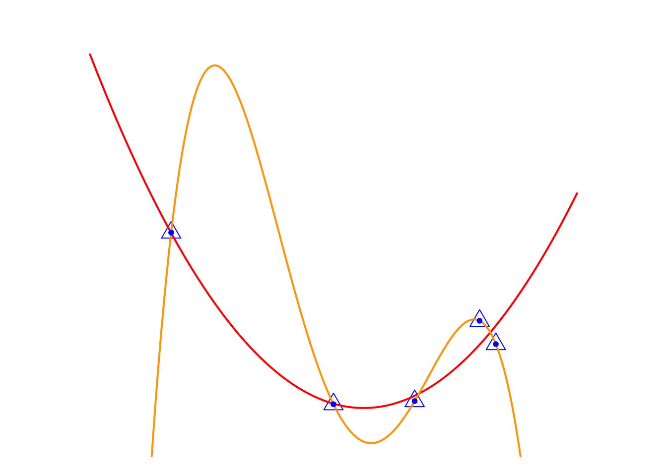
In the previous lecture, we used it to introduce the problem of overfitting. Now, let’s look at this issue from the perspective of feature selection. Do you remember the main challenge of the feature mapping idea? That’s right—choosing an appropriate feature mapping is the key challenge. In other words, here we are considering selecting some suitable variables from a set of feature variables, \(\{x, x^2, x^3, x^4\}\), to predict the \(y\) variable.

Now, let’s take a look at the relationship between the two models. The Orange Model can be viewed as the full model, \[ y_i=w_0+w_1x_i+w_2x_i^2+w_3x_i^3+w_4x_i^4+\epsilon_i \] The ideal model, Red Model, \(y_i=w_0+w_1x_i+w_2x_i^2+\epsilon_i\), can be seen as a special case of Orange Model, or the full model with an added constraint on model parameters, i.e. \[ \textcolor[rgb]{1.00,0.00,0.00}{\text{Model}} = \textcolor[rgb]{1.00,0.50,0.00}{\text{Model}} + \text{Constraint} (w_3=w_4=0) \] If the Red Model is considered as one of the candidate models in the model selection process, we can gain an insight: candidate models can be expressed as \[ \textcolor[rgb]{1.00,0.00,0.00}{\text{Candidate Models}} = \textcolor[rgb]{1.00,0.50,0.00}{\text{Full Model}} + \text{Constraint}(\textbf{w}). \] Of course, this Constraint, \(w_3=w_4=0\), is too specific. What we aim for is to use a single expression to represent a set of candidate models and then select the best one through an algorithm. Let’s look at another example. In the remark from Section 3.2.1, we mentioned that to reduce the computational cost in the best subset algorithm, we can set an upper limit on the number of features, \(k_{max}\), included in the model. It can be expressed as \[ \text{Constraint}(\textbf{w}): \sum_{j = 1}^4 \textbf{1} \{ w_j \neq 0 \} \leq 3 \]

This constraint can be interpreted as the total number of non-zero parameters being less than or equal to 3. In a figurative way, it’s like saying to the cute little parameters, “Hey, our data is limited, so only three of you can have non-zero values!” From this perspective, the restriction in our formula represents the “budget” for non-zero parameter values. If you agree with me, let’s rewrite the formula of candidate models as

\[ \textcolor[rgb]{1.00,0.00,0.00}{\text{Candidate Models}} = \textcolor[rgb]{1.00,0.50,0.00}{\text{Full Model}} + \textbf{Budget}(\textbf{w}). \] What practical significance does this formula have? It’s significant because if we can represent a set of candidate models with a single formula, we can substitute it into the loss function when estimating model parameters. This allows us to frame the model selection problem as an optimization problem.

Note: The “budget” term is a function of model parameters, and it is referred to as penalty term in the formal language.

In this way, we may have the opportunity to develop a smart algorithm to find the optimal model, rather than relying on brute-force methods like best subset selection, see the figure below.

\[ \begin{matrix} \text{Best subset selection:} \\ \\ \mathcal{L}_{mse}(y_i, w_0+w_1x_i) \\ \mathcal{L}_{mse}(y_i, w_0+w_1x_i+w_2x_i^2) \\ \mathcal{L}_{mse}(y_i, w_0+w_1x_i+w_2x_i^2+w_3x_i^3) \\ \mathcal{L}_{mse}(y_i, w_0+w_1x_i+w_2x_i^2+w_4x_i^4) \\ \vdots \\ \end{matrix} \]

\[ \begin{matrix} \text{Regularization methods:} \\ \\ \\ \\ \mathcal{L}_{mse}(y_i, f(x_i，\textbf{w})+\text{Budget}(\textbf{w})) \\ \\ \\ \\ \end{matrix} \]

where \(\mathcal{L}_{mse}\) is the mse-loss function and \(f(x_i)\) is the full model, \[ f(x_i)=w_0+w_1x_i+w_2x_i^2+w_3x_i^3+w_4x_i^4+\epsilon_i \] LHS: In best subset selection, we need to solve multiple optimization problems, one for each candidate model. RHS: However, in regularization methods, with the help of the budget term, we only need to solve a single integrated optimization problem.

How exactly does regularization methods work? Let’s discuss it further in the next subsection.

3.3.2 Ridge Regression

Overall, ridge regression belongs to the family of regularization methods. It represents the budget term using the \(l_2\)-norm, which has favorable mathematical properties, making the optimization problem solvable. To better illustrate this, let’s first revisit the previous discussion and express the best subset selection method using an optimization formula.

\[ \begin{matrix} \min_{\textbf{w}} & \sum_{i=1}^n (y_i- w_0+w_1x_i+w_2x_i^2+w_3x_i^3+w_4x_i^4)^2 \\ s.t. & \sum_{j = 1}^4 \textbf{1} \{ w_j \neq 0 \} \leq 3 \end{matrix} \] i.e. consider a constraint while minimizing the MSE loss. However, this constraint lacks favorable mathematical properties, such as differentiability, making it impossible to solve the optimization problem. Therefore, we need to modify the constraint. The \(l_2\)-norm is a good option, \[ \sum_{j = 1}^4 w_i^2 \leq 3 \] With the \(l_2\)-norm constraint, we can modify the problem as a ridge regression problem \[ \begin{matrix} \min_{\textbf{w}} & \sum_{i=1}^n (y_i- w_0+w_1x_i+w_2x_i^2+w_3x_i^3+w_4x_i^4)^2 \\ s.t. & \sum_{j = 1}^4 w_j^2 \leq C \end{matrix} \] Here, \(C\) represents a budget for all the parameter values and will be treated as a hyper-parameter. When \(C\) is large, we have a generous budget and will consider more complex models. Conversely, when \(C\) is small, our choices are limited, and the resulting model will have lower complexity.

This formulation of the optimization problem is typically called the budget form, and we need to solve it using the method of Lagrange multipliers. The optimization results are the regression coefficients of ridge regression.

It also has an equivalent form, known as the penalty form

\[ \min_{\textbf{w}} \left\{ \sum_{i=1}^n (y_i- w_0+w_1x_i+w_2x_i^2+w_3x_i^3+w_4x_i^4)^2 + \lambda \sum_{j = 1}^4 w_j^2 \right\} \]

In this form, \(\lambda\) is the given penalty weight, which corresponds to the hyper-parameter \(C\), but with the opposite meaning. When \(\lambda\) is large, to minimize the loss function, we need to consider smaller model parameters, meaning our budget \(C\) is small, and as a result, we obtain a model with lower complexity. Conversely, when \(\lambda\) is small, our budget \(C\) is large, and we end up with a model of higher complexity. Let’s see the following example.

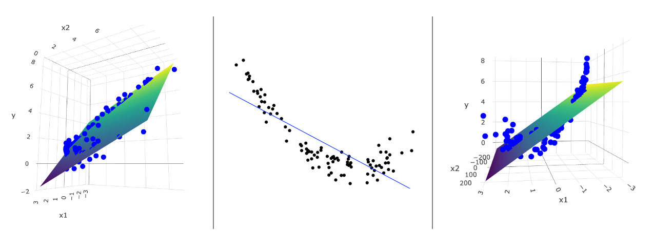
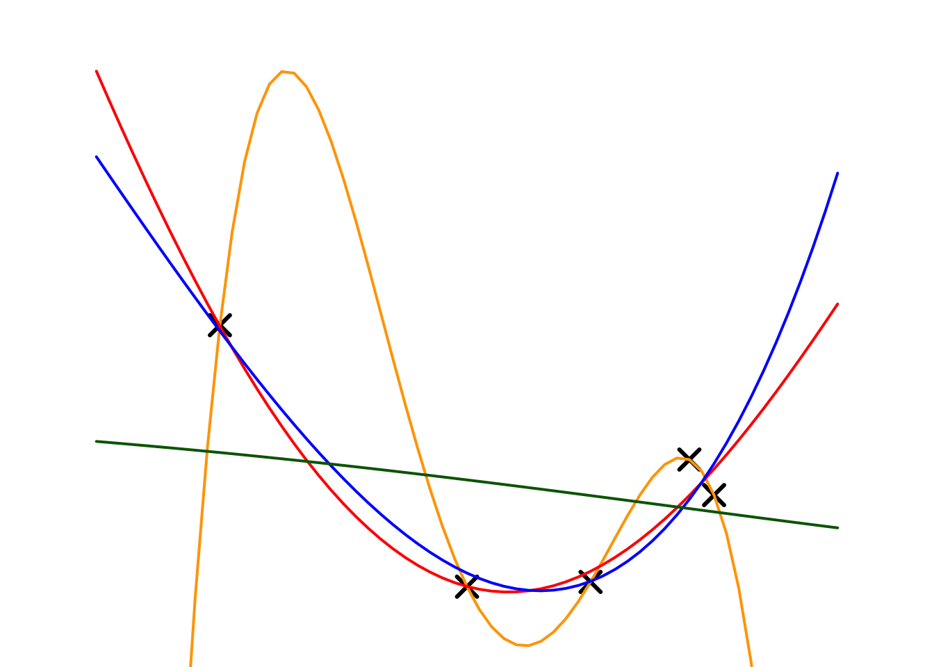
Example:

Next, we will apply ridge regression to our toy example. Here, we choose the full model as a 4th-order polynomial regression and experiment with different penalty parameters (\(\lambda\)). The fitting results and estimated regression coefficients are shown below.

Models	\(\lambda\)	\(w_0\)	\(w_1\)	\(w_2\)	\(w_3\)	\(w_4\)
Orange	0	-22.438	44.151	-25.390	5.681	-0.438
Red	0.001	3.624	-2.307	0.195	0.051	-0.005
Blue	0.01	2.931	-1.463	0.027	0.022	0.002
Green	10	0.626	-0.083	-0.007	0.000	0.000

The table summarizes the results of a ridge regression experiment, illustrating the relationship between the penalty parameter \(\lambda\) and model complexity. As \(\lambda\) increases, the penalty for larger parameter values grows stronger, resulting in smaller coefficients for all parameters (\(w_0, w_1, w_2, w_3, w_4\)).

For example, with \(\lambda = 0\) (orange model), the model has no penalty, leading to large parameter values and a highly complex model. As \(\lambda\) increases to \(0.001\) (red model) and \(0.01\) (blue model ), the parameters shrink, indicating a reduction in model complexity. When \(\lambda = 10\) (green model), most parameter values approach zero, yielding a very simple model.

This experiment demonstrates that ridge regression effectively controls model complexity through the hyper-parameter \(\lambda\), where larger \(\lambda\) values correspond to simpler models with lower complexity.

We can also observe that as \(\lambda\) increases, the estimated regression coefficients continue to shrink. This is why the ridge regression model is also referred to as a shrinkage method. It is primarily used as a robust regression model to address over fitting issues.

If we wish to use it as a feature selection tool, an additional threshold value needs to be set. For instance, feature variables corresponding to regression coefficients smaller than \(0.01\) can be excluded. For the purpose of feature selection, there are other regularization methods available, such as the LASSO, which we will discuss next.

3.3.3 LASSO

The LASSO (Least Absolute Shrinkage and Selection Operator) is a regularization method that adds an \(l_1\)-norm penalty to the loss function, encouraging sparsity in the model coefficients. This unique property enables LASSO to perform both shrinkage and feature selection simultaneously, making it a powerful tool for high-dimensional data analysis.

Compared to the \(l_2\)-norm penalty used in ridge regression, LASSO employs the \(l_1\)-norm to calculate the coefficients budget, which is \[ \sum_{j = 1}^p |w_j| \leq C \] So, LASSO problem can be expressed as in the budget form, \[ \begin{matrix} \min_{\textbf{w}} & \sum_{i=1}^n (y_i- w_0+w_1x_i+w_2x_2+\dots+w_px_p)^2 \\ s.t. & \sum_{j = 1}^p |w_j| \leq C \end{matrix} \] or the penalty form \[ \min_{\textbf{w}} \left\{ \sum_{i=1}^n (y_i- w_0+w_1x_i+w_2x_2+\dots+w_px_p)^2 + \lambda \sum_{j = 1}^p |w_j| \right\} \]

Similar to Ridge regression, the budget parameter \(C\) and penalty parameter \(\lambda\) here are treated as hyper parameters. They carry the same significance as the hyper parameters in Ridge regression. By solving this optimization problem, we can obtain the estimated LASSO parameters.

In the laboratory exercises, we will find that, unlike the shrinkage results of ridge regression, the estimates from LASSO are called sparse results, meaning that most regression coefficients are zero, while a few coefficients are non-zero. Therefore LASSO is also called Sparse method. This characteristic of LASSO makes it an important tool for feature selection.

The following diagram conceptually explains why LASSO produces sparse results.

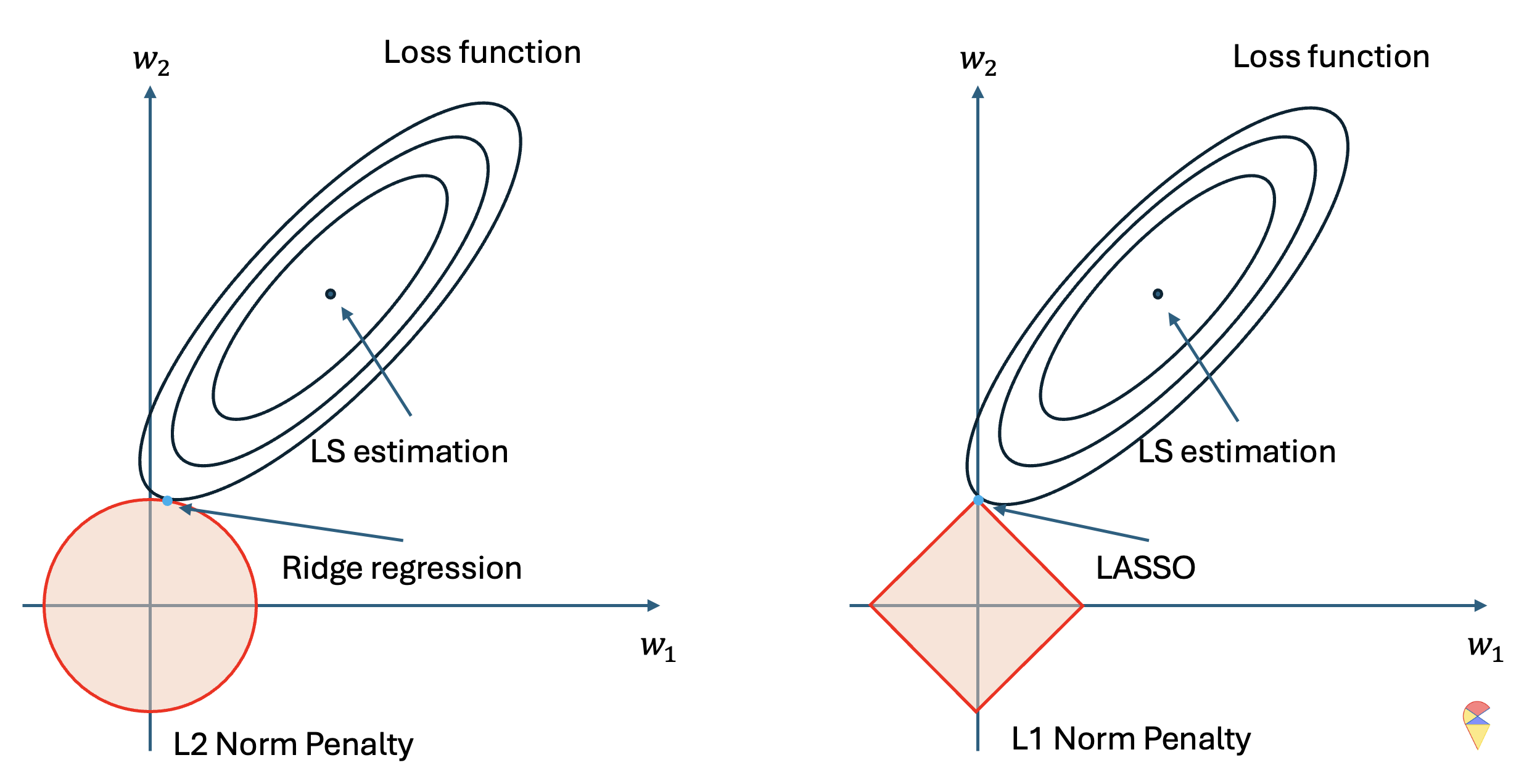
The left and right sides represent the optimization problem for the same regression model. We can see that in this optimization problem, we have two optimization variables, and the ellipse represents the contour plot of the loss function for the regression problem, where the closer to the center, the lower the loss value. Therefore, without considering the pink figure, the dark blue point represents the optimal solution to the optimization problem, which is the least squares solution, i.e., the regression coefficients for the regular regression model.

However, when we consider the constraint, we need to limit the possible points to a specific region, which is the pink area. On the left, the circle represents the feasible region for the two coefficients under the \(l_2\) norm constraint, while on the right, the diamond shape represents the feasible region for the two coefficients under the \(l_1\) norm constraint. In other words, we can only consider the optimal solution within the pink region. As a result, the optimal solution is the light blue point, which is the point closest to the minimum loss function value within the feasible region.

From the above diagram, it is clear that the geometric characteristics of the two penalty functions determine the nature of their solutions. Under the \(l_2\) norm, the solution is closer to the y-axis, indicating that, due to the penalty term, the estimate of \(w_1\) undergoes shrinkage toward zero. Under the \(l_1\) norm, the solution lies exactly on the y-axis, meaning that, due to the penalty term, \(w_1\) becomes exactly zero. This explains why the \(l_1\) norm leads to sparse results, while the \(l_2\) norm leads to shrinkage results.

Lecture 6 Homepage