5.2 Nonlinear Regression Models
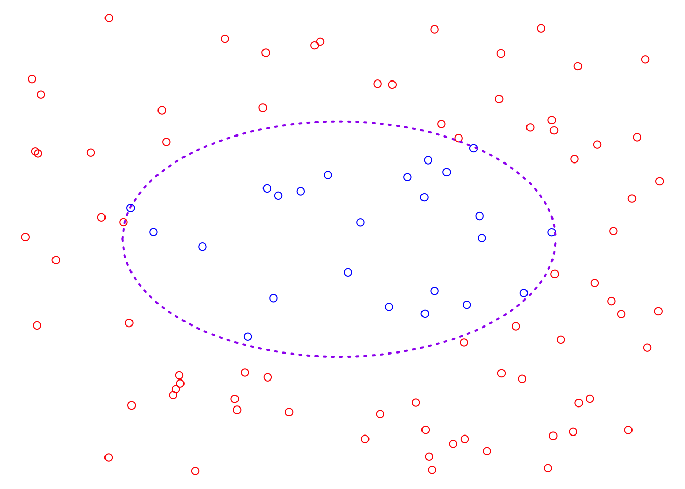
So far, we have studied two linear models, however, it is by no means enough to solve the problems in reality. For example, the plot below displays a classification problem, and clearly, we cannot find a suitable linear classifier. In other words, we cannot identify a straight line that can divide this 2D feature space in such a way that the two classes of sample points are located on opposite sides of the line. At the same time, through data visualization, we can roughly observe that the boundary between the two classes is an ellipse. Therefore, to address this problem, we must extend our linear model to find a solution.
5.2.1 Basic ideas of Non-linear Extension
Nonlinear models are not the focus of our course, however, here we can explore the basic approach to finding nonlinear models, that is feature mapping. Feature mapping involves the basic idea of introducing new variables by transforming the original feature variables with functions. This expands the original feature space, allowing the exploration of potential linear solutions within the augmented feature space. Let’s start with the toy example of classification problem above.
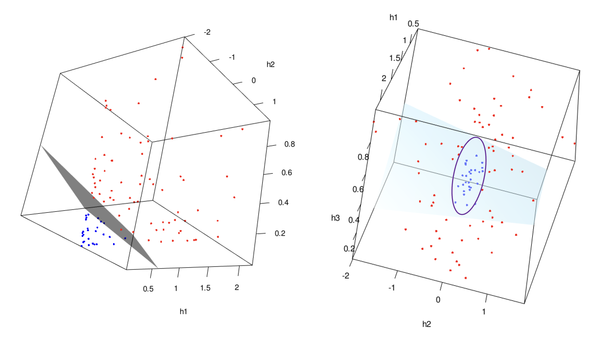
In the classification problem, we can consider three new variables \(\left(h_1 = x_1^2, h_2 = \sqrt{2}x_1x_2, h_3 = x_2^2 \right)\) instead of the two original variables \(x_1, x_2\). The new data set is visualized in the following 3D plot.
If you rotate the 3D scatter plot above, you may notice that the same set of observed cases becomes linearly separable in the new feature space, see the LHS of plot below. For example, we can train an LDA classifier using three new feature variables, \(\left(h_1, h_2, h_3 \right)\). The decision boundary of this classifier would correspond to the gray plane in the 3D space. By building the new feature space, the previously non-linearly separable data points may now become linearly separable, allowing the LDA classifier to effectively separate the two classes. Also, if we change the direction of our view, the linear model in the augmented feature space is eventually a nonlinear model in the original space, see the LHS of the plots below.
We can refer to this idea as the feature mapping idea. In simple terms, we need to find an appropriate new space, which we call the augmented feature space, and train our linear model within it. This augmented feature space is entirely determined by a transformation function, \(\phi(\textbf{x}) : \text{p-D space} \to \text{q-D space}\) which we refer to as feature mappings.
This concept plays a significant role in machine learning, and almost all advanced nonlinear models are based on this idea. For example:
- Before deep learning dominated AI, the Support Vector Machine (SVM) applied this idea indirectly through the kernel function. The kernel allows the SVM to operate in a higher-dimensional space without explicitly computing the coordinates in that space.
- In the world of ensemble methods, which dominate structured data tasks, each single model can be seen as a form of feature mapping.
- In the foundation deep learning model, the neural network, the chain of transformations through neurons can also be seen as a feature transformation.
This idea of transforming data into a higher-dimensional space (whether directly or indirectly) enables models to handle complex, nonlinear relationships that would otherwise be difficult to capture in the original space.
5.2.2 Polynomial Regression Model
In this section, we will introduce a nonlinear regression model using the feature mapping idea, specifically focusing on polynomial regression. Let’s begin by looking at a simple example.
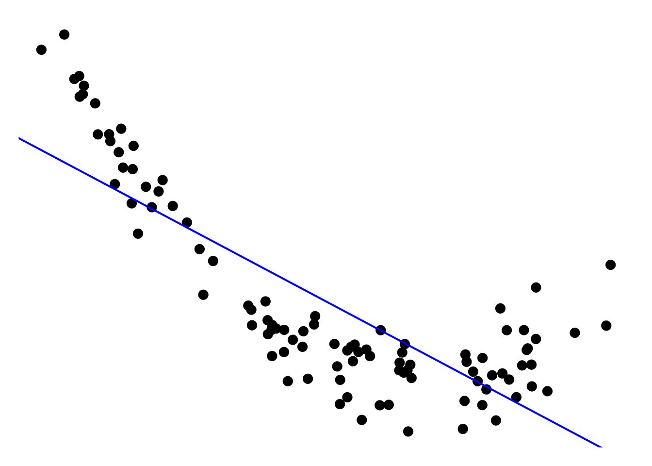
In this example, we are dealing with a nonlinear regression problem, where the relationship between the feature variable and the target variable is clearly nonlinear. A linear model would not provide satisfactory results because it assumes a straight-line relationship between the features and the target. As you can see, the blue line in the plot, i.e. the simple linear model has totally unacceptable performance on the whole domain. However, by using the feature mapping idea, we can transform the feature space into a higher-dimensional space, where the relationship becomes linear, making it possible to apply linear regression successfully. To do so, we introduce the augmented feature space by the feature mapping \(\phi(x) = (x, x^2)\), i.e. a mapping from 1D to 2D, see the 3D scatter plot below
You can see that all the points stand on a plane in the augmented space which means that we can find a linear model, i.e. \[ y = w_0 + w_1x + w_2x^2, \] to solve the problem.
Remark: I believe you can see that the choice of feature mapping, \(\phi()\), or basis functions, is extremely important. If we choose an inappropriate set of feature mappings, we may end up with very poor results. As shown in the figure below, we apply \(\phi(x) = (x, x^5)\) to obtain the augmented feature space, then we eventually switch to another nonlinear problem. In other words, we can’t find a plane in the new space such that all the sample points roughly all stand on it. So, we naturally have the following question and we will answer it in the next lecture.
Question: How to choose an appropriate feature mapping?