Lecture 5: Regression Models
In this lecture, we discuss regression problems. First, we review the training methods of linear regression models from different perspectives. Then, a basic nonlinear extension idea is introduced, feature mapping, and use it to introduce the first nonlinear regression model, polynomial regression. Afterward, we understand polynomial regression from the perspective of basis functions, and then introduce another commonly used nonlinear model, spline regression. At the end of this lecture, we introduce a new concept, the overfitting problem. It is a core challenge in machine learning from the training perspective, and we focus on it in the next lecture.
5.1 Linear Regression Model
Unlike classification problems, the target variable in regression is continuous, but it inherits the basic idea of classification problems, which is to predict the target variable using a weighted combination of feature variables, i.e. \[ y = w_0 + w_1 x_1 + \dots w_px_p + \epsilon \] where \(\epsilon\) is a error term. The error term contains many things. It could be measurement errors, or random noise, or all the variations that can not be explained by all the feature variables. For the latest case, it also means we need more feature variables for a better prediction of the target variable.
Obviously, we have to apply some methods (algorithm) to learn the model, i.e. estimate the coefficients \(w_0, w_1, \dots, w_p\) from a data set. Here, we mainly discuss two methods, least square methods and maximum likelihood method. Eventually, the two methods are equivalent for a regression problem, however, it is still necessary to explain maximum likelihood method for understanding logistic regression in lecture 7.
5.1.1 Least Square Method
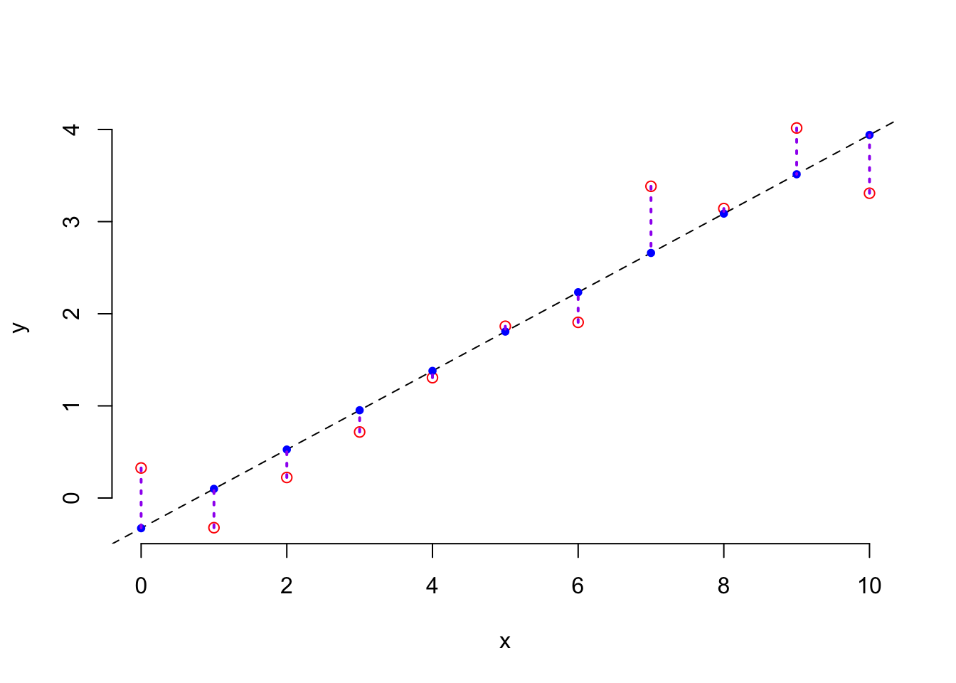
Least Square method was proposed by the famous mathematician Gauss. He applied this method for data analysis to accurately predict the time of the second appearance of the asteroid, Ceres. His idea is quite simple: to use data to find the optimal line, represented by two coefficients, in order to minimize prediction errors, see the plot below.
Suppose that we have a set of paired observations, \((y_1,x_1), \dots, (y_n, x_n)\), then the mathematical formulation is \[ \hat{w}_0, \hat{w}_1 = \arg\min_{w_0, w_1} \sum_{i=1}^n(y_i-\hat{y}_i)^2 \] where \(\hat{y}_i = w_0 + w_1x_i\).
The solution of this optimization problem is \(\widehat{w}_1=\frac{\sum_{i=1}^N(x_i-\overline{x})(y_i-\overline{y})}{\sum_{i=1}^N(x_i-\overline{x})^2}\), and \(\widehat{w}_0=\overline{y}-\widehat{w}_1\overline{x}\)
5.1.2 Matrix Form ( NE )
When we consider multiple feature variables in a linear regression model, the above calculation formula becomes somewhat cumbersome and inefficient. To compute all the regression coefficients more effectively, we typically need to consider the matrix form of the model. By expressing the linear regression model in matrix form, we can simplify the computation and make it more efficient. The model can be written as: \[ \textbf{y} = \textbf{Xw} + \epsilon \] where: - \(\textbf{y}\) is the vector of observed values (target variable), \(\textbf{y} = (y_1, \dots, y_n)^{\top}\), - \(\textbf{X}\) is the design matrix, which contains the feature variables (including a column of ones for the intercept), i.e. \[ \textbf{X}= \begin{pmatrix} 1 & x_{1,1} & \cdots & x_{1,p}\\ \vdots & \vdots & \ddots & \vdots \\ 1 & x_{n,1} & \cdots & x_{n,p} \end{pmatrix} \]
- \(\textbf{w}\) is the vector of regression coefficients, \(\textbf{w} = (w_0, w_1, \dots, w_p)^{\top}\)
- \(\boldsymbol{\epsilon}\) is the vector of errors, \(\boldsymbol{\epsilon} = (\epsilon_1, \dots, \epsilon_n)^{\top}\).
To estimate the regression coefficients , we use the least squares method, which minimizes the sum of squared errors. The solution to this optimization problem is: \[ \widehat{\textbf{w}}=(\textbf{X}^{\top}\textbf{X})^{-1}\textbf{X}^{\top}\textbf{y} \]
This formula provides an efficient way to calculate the coefficients for a linear regression model with multiple features. Using matrix operations not only simplifies the calculations but also allows for faster computation, especially when dealing with large data sets or numerous features. Thus, the matrix form of the model allows for a more streamlined approach to regression analysis, making it easier to implement and compute the necessary coefficients, particularly when working with multiple variables.
5.1.3 Maximum Likelihood Method
Different from least square method, next, we are going to reexamine the regression model from the perspective of probability models. To do so, we assume the error term \(\epsilon\) is normally distributed, \(\epsilon \sim \mathcal{N}(0, \sigma^2)\). Based on this assumption, the target variable is normally distributed conditional on feature variables. Therefore, we essentially predict the expected value of the target variable conditional on \(X_1, \dots, X_p\) as a linear model, i.e.

\[ \text{E}(Y | X_1, \dots, X_p) = w_0 + w_1 X_1 + w_2 X_2 + \dots + w_p X_p \] Based on the normality assumption, another estimation method, MLE, for coefficients can be discussed.
MLE of regression model: Under the normality assumption, we have \(y_i \sim \mathcal{N}( w_0 + w_1x_1 , \sigma^2)\). If you remember the secrete message behind the normal distribution, the likelihood of each observation, \(y_i\), is inversely proportionally to the distance to the expected value, i.e. \[ f( y_i | w_0, w_1, \sigma^2 ) \propto -(y_i - (w_0 + w_1x_1 ) )^2 \] Therefore the likelihood function of the sample \(\left\{ y_i, x_i \right\}_{i=1}^n\) is \[ \log \left( L( w_0, w_1, \sigma^2 | (y_i, x_i) ) \right) \propto -\sum_{i=1}^n (y_i - (w_0 + w_1x_1 ) )^2 \]
Notice that, on the LHS, it is sum square of residual. Therefore, minimize sum square of residuals is equivalent to maximize the log likelihood function. In other words, the two methods are equivalent.
5.1.4 Model Evaluation
Unlike classification problems, model evaluation for regression problems is quite straightforward. From the purpose of regression, our ultimate goal is to use feature variables to estimate a continuous target variable. A good regression model naturally minimizes prediction error. Therefore, we typically use the mean squared error (MSE) of the model predictions for evaluation. That is \[ \text{MSE} = \frac{1}{N} \sum_{i = 1}^N \left( y_i - \hat{y}_i\right)^2 \]
where \(\hat{y}_i\) is the prediction of the \(i\)th case, i.e. \(\hat{w}_0 + \hat{w}_1 x_{i,1} + \dots + \hat{w}_p x_{i,p}\), and therefore \(y_i - \hat{y}_i\) is the prediction error of the \(i\)th case. To gain a more intuitive understanding, people often use RMSE (Root Mean Squared Error), i.e. \(\text{RMSE} = \sqrt{\text{MSE}}\). Sometimes, people also use Mean Absolute Error (MAE) to evaluate a regression model. \[ \text{MAE} = \frac{1}{N} \sum_{i = 1}^N | y_i - \hat{y}_i| \] For all metrics, lower value indicates better model performance.
Quiz: Do you know why we don’t use the average errors, i.e. \(\frac{1}{N} \sum_{i = 1}^N \left( y_i - \hat{y}_i\right)\) to evaluate a regression model?
Tips: The simplest regression model is \(y = w_0 + \epsilon\) and the estimation is \(\hat{w}_0 = \bar{y}\), i.e. \(\hat{y} = \bar{y}\).
5.1.5 Loss function
The attentive among you may have noticed that the objective function of the least squares method in regression problems is the same as the model evaluation metric, MSE. From another perspective, we can understand the estimation of regression models as finding a set of regression coefficients that minimize the MSE. In machine learning, estimating regression coefficients is framed as an optimization problem, where MSE is interpreted as the objective function of this optimization problem, also referred to as the model’s loss function. For a regression problem, it is called MSE loss: \[ \mathcal{L} = \frac{1}{N} \sum_{i=1}^N (y_i - \hat{y}_i)^2 \] For different problem, we could have different loss functions, for example, Huber loss, cross entropy loss, hinge loss. We will explore this further in the lab exercises. This concept, connecting to Maximum Likelihood Estimation, will reappear and be discussed again in the context of logistic regression models.
5.2 Nonlinear Regression Models
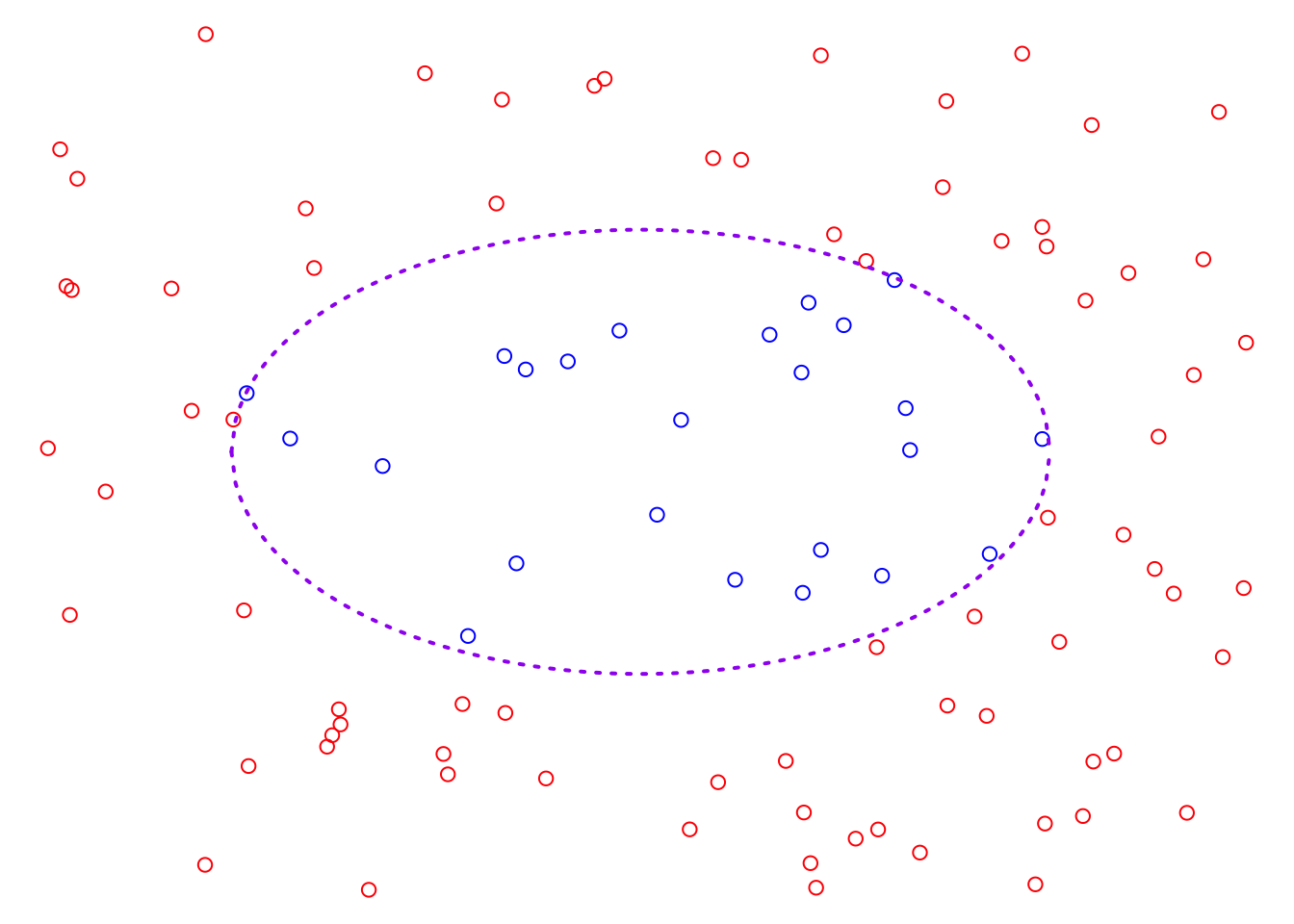
So far, we have studied two linear models, however, it is by no means enough to solve the problems in reality. For example, the plot below displays a classification problem, and clearly, we cannot find a suitable linear classifier. In other words, we cannot identify a straight line that can divide this 2D feature space in such a way that the two classes of sample points are located on opposite sides of the line. At the same time, through data visualization, we can roughly observe that the boundary between the two classes is an ellipse. Therefore, to address this problem, we must extend our linear model to find a solution.
5.2.1 Basic ideas of Non-linear Extension
Nonlinear models are not the focus of our course, however, here we can explore the basic approach to finding nonlinear models, that is feature mapping. Feature mapping involves the basic idea of introducing new variables by transforming the original feature variables with functions. This expands the original feature space, allowing the exploration of potential linear solutions within the augmented feature space. Let’s start with the toy example of classification problem above.
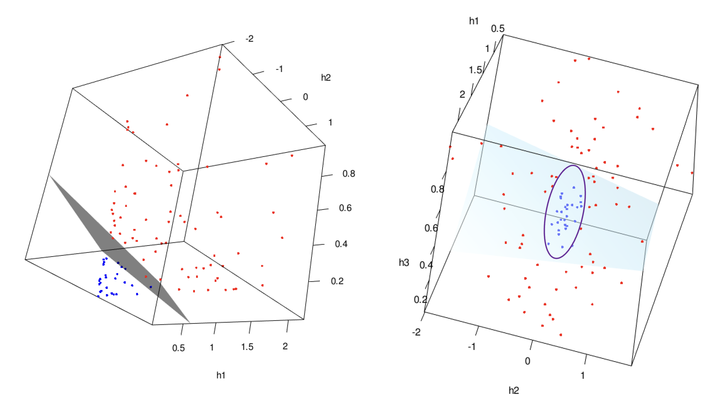
In the classification problem, we can consider three new variables \(\left(h_1 = x_1^2, h_2 = \sqrt{2}x_1x_2, h_3 = x_2^2 \right)\) instead of the two original variables \(x_1, x_2\). The new data set is visualized in the following 3D plot.
If you rotate the 3D scatter plot above, you may notice that the same set of observed cases becomes linearly separable in the new feature space, see the LHS of plot below. For example, we can train an LDA classifier using three new feature variables, \(\left(h_1, h_2, h_3 \right)\). The decision boundary of this classifier would correspond to the gray plane in the 3D space. By building the new feature space, the previously non-linearly separable data points may now become linearly separable, allowing the LDA classifier to effectively separate the two classes. Also, if we change the direction of our view, the linear model in the augmented feature space is eventually a nonlinear model in the original space, see the LHS of the plots below.
We can refer to this idea as the feature mapping idea. In simple terms, we need to find an appropriate new space, which we call the augmented feature space, and train our linear model within it. This augmented feature space is entirely determined by a transformation function, \(\phi(\textbf{x}) : \text{p-D space} \to \text{q-D space}\) which we refer to as feature mappings.
This concept plays a significant role in machine learning, and almost all advanced nonlinear models are based on this idea. For example:
- Before deep learning dominated AI, the Support Vector Machine (SVM) applied this idea indirectly through the kernel function. The kernel allows the SVM to operate in a higher-dimensional space without explicitly computing the coordinates in that space.
- In the world of ensemble methods, which dominate structured data tasks, each single model can be seen as a form of feature mapping.
- In the foundation deep learning model, the neural network, the chain of transformations through neurons can also be seen as a feature transformation.
This idea of transforming data into a higher-dimensional space (whether directly or indirectly) enables models to handle complex, nonlinear relationships that would otherwise be difficult to capture in the original space.
5.2.2 Polynomial Regression Model
In this section, we will introduce a nonlinear regression model using the feature mapping idea, specifically focusing on polynomial regression. Let’s begin by looking at a simple example.
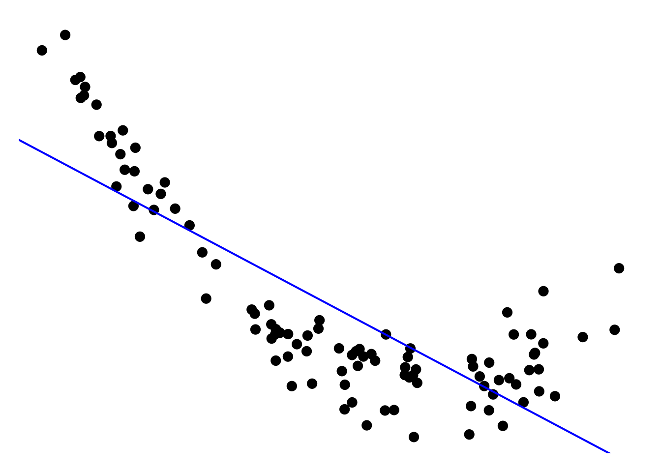
In this example, we are dealing with a nonlinear regression problem, where the relationship between the feature variable and the target variable is clearly nonlinear. A linear model would not provide satisfactory results because it assumes a straight-line relationship between the features and the target. As you can see, the blue line in the plot, i.e. the simple linear model has totally unacceptable performance on the whole domain. However, by using the feature mapping idea, we can transform the feature space into a higher-dimensional space, where the relationship becomes linear, making it possible to apply linear regression successfully. To do so, we introduce the augmented feature space by the feature mapping \(\phi(x) = (x, x^2)\), i.e. a mapping from 1D to 2D, see the 3D scatter plot below
You can see that all the points stand on a plane in the augmented space which means that we can find a linear model, i.e. \[ y = w_0 + w_1x + w_2x^2, \] to solve the problem.
Remark: I believe you can see that the choice of feature mapping, \(\phi()\), or basis functions, is extremely important. If we choose an inappropriate set of feature mappings, we may end up with very poor results. As shown in the figure below, we apply \(\phi(x) = (x, x^5)\) to obtain the augmented feature space, then we eventually switch to another nonlinear problem. In other words, we can’t find a plane in the new space such that all the sample points roughly all stand on it. So, we naturally have the following question and we will answer it in the next lecture.
Question: How to choose an appropriate feature mapping?