# randomly generate 5000 numbers taking values 0 or 1 and save in x
set.seed(8312)
x = rbinom(1000,1,0.5)
# calculate the cumulated ratio
ratio = cumsum(x)/(1:1000)
plot(ratio, type = "l")
abline(h = 0.5, col = "red")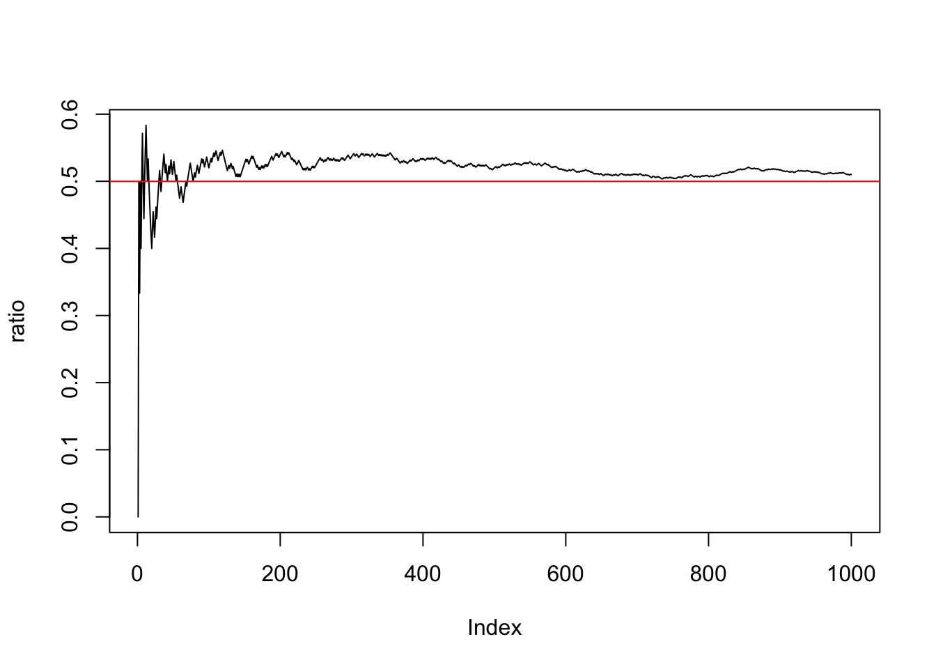
Machine learning is essentially about finding methods for making decisions, and the best way to make decisions is based on assessing the probability (or likelihood) of potential outcomes. Therefore, probability theory has undoubtedly become a fundamental tool in this field.
In this lecture, we will cover the fundamental concepts of probability theory. To make this note self-contained, I will start from scratch. The benefit of this approach is that we can gradually build on each concept in a coherent manner. However, there may be some topics that we won’t use in this course, so I will list the most important aspects separately at the end. If you have already studied probability theory, you can treat this as a quick review. I will do my best to provide you with an intuitive picture of probability theory. If you feel this isn’t necessary, you can also skip ahead to the exercises.
Before we begin, I want to emphasize something important: probability models exist solely within our rational world. They are summaries of patterns in observational data, rather than replicas of real-world phenomena. No probability model can perfectly replicate reality, but it can help us solve real-world problems. As the statistician Box famously said, “All models are wrong, but some are useful.” I highly recommend you take a moment to read a mini note, it may open a door to a whole new perspective for you.
(WBPA) The tools provided in this lesson are a type of soft tool. They may not help you directly with how to use the software, but they can offer you a way of thinking. A good understanding of them will make things easier for your studies not only in this course but also for all your data science knowledge.
Early on people realized that there are many things in the real world where the outcome is uncertain, such as one doesn’t always get a head when flipping a coin, or doesn’t always get a certain number when throwing a dice, and so they refer to this kind of event as random event. At the same time, mathematicians also had found that the percentage of getting heads always seems to be close to \(0.5\) when they repeatedly flip an even coin. The following r codes simulate this process:
# randomly generate 5000 numbers taking values 0 or 1 and save in x
set.seed(8312)
x = rbinom(1000,1,0.5)
# calculate the cumulated ratio
ratio = cumsum(x)/(1:1000)
plot(ratio, type = "l")
abline(h = 0.5, col = "red")
0.5, that is 1/2, has different meanings for its numerator and denominator; the denominator is the number of all possible outcomes (Head or Tail), while the numerator is the number of outcomes included in this event. Thus, mathematicians defined the first probability model in which the possibility of a random event occurring can be quantified by the ratio of the number of outcomes associated with the event to the number of all possible ones. Meantime, we refer to this measure of possibility as the probability of an event.
\[
\Pr \left( \text{Event} \right) = \frac{\text{number of outcomes associated with the event}}{\text{total number of all possible outcomes}}
\] In the coin example, all possible outcomes are \(H\) and \(T\), and the outcome associated with the event, getting a head, is \(H\). So, the probability that get a head when flip a coin is \[
\Pr(\text{Get a head when flip a coin}) = \frac{1}{2}
\] Since the number of outcomes associated with the event is always less than the total number of all possible outcomes, the probability defined by this model is always a number between 0 and 1, which fits our intuitions.
Based on this model, one can easily quantify the possibility of an event if one gets the number 3 when throwing a dice as \(1/6\). Before providing more examples, I have to emphasize that probability is a mathematical concept that only exists in our rational world. That is, you can only get a number which is 3 or not 3 after throwing a dice. Also, even if you throw a die over and over again for the rest of your life, the number of times you get a 3 as a percentage of your total throws will only be very close to \(1/6\).
( NE ) Let’s explore some more complex examples. First, what is the probability that you get a number less than 5 by throwing a dice? Using the model above, the total number of outcomes of throwing a dice is 6 and there are 4 potential outcomes all satisfy this condition, therefore this probability is \(2/3\). Second, what is the probability that you get 2 heads after flipping a coin 6 times? Again, the total number of possible outcomes is \(2^6\) and the number of outcomes satisfying this condition is \(15\), therefore the probability of this event is \(0.234375\). Obviously, the second example is harder than all the examples before, and you probably need some knowledge of permutations and combinations to understand the meaning of numbers \(2^6\) and \(15\). However, this is not the main purpose here. Also, calculating such numbers is not essential to understanding the probability model. Of course, if you’re interested in these types of questions, consider solving some problems from a book on probability theory, which is a good mental exercise. For example, you might think carefully about why a full house can beat a flush in Poker? (ToDo4Sia: Write a note discussing how you teach your son about permutations and combinations.)

Discussing the probability notion for events can often be cumbersome. For example, in the coin example, we have to write texts to represent it. To simplify the expression, we can use a capital letter \(X\) to represent the result of flipping a coin. It has two possible values, \(0\) and \(1\) which indicate getting a Tail and a Head respectively. Then the probability of that event can be represented as \[ \Pr(X = 1) \] This letter \(X\) is so powerful that it encompasses not only the two possible outcomes of one flipping but also represents all potential results each time you flip this coin. We call this letter \(X\) as a random variable which can be understood as a description of the results of a certain experiment. Conventionally, it is usually presented by a uppercase letter and we use lowercase letter, e.g. \(x\), to represent its realization or observation.
Note: the mathematical definition of a random variable goes beyond this and is much more profound; however, this understanding of random variables is sufficient for practical applications.
If the role of a random variable were merely to use a symbol to represent an experimental outcome, it wouldn’t be nearly as compelling. Its essence lies in its distribution. Through the distribution of a random variable, we can abstract the common features of a wide range of random events. For example, consider \(X\) in the context of a coin toss. If we specify that \(X\) takes the value 1 with a fixed probability \(\pi\) and 0 with a probability of \(1 - \pi\), we obtain a random variable with a specific distribution, commonly referred to as a binary distribution or Bernoulli distribution random variable. It can be denoted as \(X \sim \text{Ber}(\pi)\), and its distribution can be simply described as the evaluation of the probability for each possible outcome, i.e.

This information of distribution also can be represented by a formula,
\[ \Pr(X = k) = \pi^k(1-\pi)^{1-k} \] where the possible value of \(k\) is 0 and 1, and \(0<\pi<1\). It is called probability mass function (p.m.f).
In this way, the symbol \(X\) becomes much more powerful. The Random variable and its distribution can help us get away from the whole coin-flip thing. The symbol \(X\) is elevated, and it becomes a probabilistic model. It can not only represent the random experiment of flipping a coin but also depict the probability of randomly selecting a man in Umeå city center, or describe the incidence of a certain disease within a specific population over a certain time period in a given region.
Another example: One also can define a random variable \(Y\) denotes the result of throwing a dice, then it has 6 possible values, \(1\) to \(6\). Since the probabilities of getting all possible values are equal, \(1/6\), it is called the discrete uniform distribution. ( PA ) The p.m.f is \[ \Pr(Y = k) = 1/6 \] where \(k = 1,2,\dots,6\). There aren’t necessarily only six possible outcomes; you can increase the number of possible values, allowing this probabilistic model to cover a broader range of random phenomena.
More possibilities, for example, one can use \(Z\) to denote a random variable that presents the number of accidents in a certain time period, for example, the number of traffic accidents in certain area in one month. In this case, the possible values should be \(1,2,3,4,\dots\). From this phenomenon, we can abstract the Poisson distribution which models the number of times an event occurs in a fixed interval of time or space, under the conditions. The p.m.f is leave to you to explore.
Random variable with certain distribution also can help us simplify the calculation of the probability of an event. Let’s see the next example, Binomial distribution, denoted as \(X \sim \text{Bin}(N,p)\). The random variable \(X\) presents the number of positive results among \(N\) independent binary results experiment. The probability that getting a positive result in one experiment is \(p\). Obviously, the possible values of \(X\) are integers from \(0\) to \(N\), and the distribution can be represented as \[ \Pr(X = k) = \frac{N!}{k!(N-k)!} p^{k}(1-p)^{N-k} \] where the exclamation sign denotes factorial, i.e. \(N!=N(N-1)(N-2)\dots1\). It is easy to see the probability of the relatively complicated random event discussed before, you get \(2\) heads after flipping a coin \(6\) times, which can be calculated by this distribution. We can define a random variables the number of getting heads after flipping a coin \(6\) times, so \(X \sim \text{Bin}(6,0.5)\). Replacing \(N=6\), \(p=0.5\), and \(k=2\) in the formula above, one can easily verify \(\Pr(X=2) = 0.234375\).
We have introduced the most basic elements of probability theory, namely random variables and their distributions. Now, I have a question to you. Suppose we have two binomial distributed random variables, \(X_1 \sim \text{Bin}(10, 0.1)\) and \(X_2 \sim \text{Bin}(3, 0.7)\) , can we compare them? (You can hover your cursor on \(X_1\) and \(X_2\) to get the meaning of them.) Well, the two random variables have different potential outcome, for \(X_1\), you might get a integer from \(0\) to \(10\), but only three possible values, \(0, 1, 2, 3\) for \(X_2\). Apparently, it is not comparable. Then can we compare their observed values? It doesn’t seem that simple neither. One is an experiment with a low success rate conducted 10 times, while the other has a high success rate but we only conduct it 3 times, so it’s hard to say which will have a higher number of successes. Let’s explore the answer in a straightforward way by actually generating two random numbers from their respective distributions and comparing them.
If you run the code above multiple times, you’ll get both TRUE and FALSE, but you may feel that the realization of \(X_2\) is often higher than the realization of \(X_1\). To verify our intuition, we can repeatedly run the code above and record the result each time. By doing this 1000 times, we can see the percentage of cases where the value of \(X_2\) is greater than the value of \(X_1\).
res = numeric(1000)
for(i in 1:1000){
  X1 = rbinom(1, prob = 0.1, size = 10)
  X2 = rbinom(1, prob = 0.7, size = 3)
  res[i] = ifelse(X2>X1,1,0)
}
print(paste0("The proportion of times X2>X1 is ", sum(res)/10,"%"))
[1] "The proportion of times X2>X1 is 69.5%"Indeed, we often observe that the value of \(X_2\) is greater than \(X_1\). However, is there a way to reach a conclusion directly without relying on experiments? Or perhaps, can we explain this phenomenon using mathematical language? We then need to introduce another important concept, the expected value of a random variable. The expected value of a random variable is very similar to the concept that you are very familiar with, that is average value. If I ask you how often do you go to IKSU per week? Then most likely, you will answer me that you go to IKSU, on average, 3 times per week, since the number of visiting IKSU (the largest sports center in Umeå) per week is not a certain number (you often go there 3 times, but not always, for example, you are sick or have an important exam to prepare). Let me show you the number of my IKSU visits in the last 10 weeks. \[ 3,5,3,2,2,4,5,3,3,4 \]
We all know that the average value can be \[ \frac{3+5+3+2+2+4+5+3+3+4}{10} = 3.4 \] Of course, it is a super easy calculation, but let’s have a close look at it. This calculation can be represented as \[ \frac{2 \times 2 + 4\times3 + 2\times4 +2\times 5 }{10} = 0.2 \times 2 + 0.4 \times 3 + 0.2 \times 4 + 0.2 \times 5 = 3.4 \]
Notice that the decimal in front of each integer, the possible value, is the percentage of the corresponding value that happened in the last ten weeks. In the rational world, if you still remember it, the percentage is replaced by the probability. Therefore, the definition of expected value is defined as the weighted sum of all possible values, and the weights are the corresponding probabilities. In a mathematical notation, the expected value of a random variable is presented as \[ \text{E}(X) = \sum_{k} k \Pr (X = k) \] We can see that the expected value of a binary distributed random variable and a binomial distributed random variable is \(p\) and \(Np\) respectively. It is a good exercise to verify it. Now, we can turn back to the question at the beginning. By simple calculation, we can see that \[ \text{E}(X_2) = 3\times0.7 = 2.1 > \text{E}(X_1) = 10\times0.1 = 1 \] The expected value satisfies linearity. Suppose \(a\) and \(b\) are constant numbers and \(X\) is a random variable, then \(\text{E}(aX+b) = a \text{E}(X) + b\). In other words, linearity means the expectation operator and the linear operator (scalar multiplication and addition) are exchangeable, i.e. \[ \text{E} \left(\sum_{i=1}^n a_iX_i\right) = \sum_{i=1}^n a_i\text{E}(X_i) \]
The expected value can help us determine the size of the “common” value of a random variable so that we can compare two random variables. One can also compare two random variables from another dimension, which is “value stability”. For example, we have two coins, one is even and the other is so uneven that there is a very high probability, 90%, of getting Heads. Then imagine that if we flip two coins repeatedly, we will get many heads for the uneven coin and occasionally get Tails; but for the even coin, we will get the same number of heads and tails with high probability. From the perspective of taking values, the values of uneven coins are very stable, while those of uniform coins are not. The stability of a random also refers to variation. High variation means low stability. The two things can be quantified by the variance.
The variance of a random variable \(X\) is defined as \[ \text{Var}(X) = \text{E}(X - \text{E}(X))^2 \]
This formula is very intuitive. First, we calculate the most frequently occurring value of this random variable, \(\text{E}(X)\), and then compare it with any \(X\) by taking the difference. Finally, we calculate the average of the squares of this difference. If this random variable has stable values, then the value of \(X\) should often stay around the expected value, therefore \(X - \text{E}(X)\) will generally be very small; conversely, if it varies significantly, it will be generally large, which aligns perfectly with our initial intention.
Based on this definition, one can easily verify the variance of a binary distributed random variable and a binomial distributed random variable is \(p(1-p)\) and \(np(1-p)\) respectively. In the example above, the variance of the even coin is \(0.25\), but the uneven is \(0.09\).
Different from the expected value, variance doesn’t satisfy the linearity, i.e. the variance operator and the linear operator are not exchangeable. However, it satisfies the following rules, \[ \text{Var}(aX+b) = a^2\text{Var}(X) \]
Based on the results above, we can easily find that a special linear combination, \(\left( X-\text{E}(X) \right)/\sqrt{\text{Var}(X)}\), produces a standardized random variable, i.e. mean zero and variance 1.
Let’s think about a question like this. The basic conditions are presented in the following picture. Suppose we want to randomly pick a box and then randomly take out a fruit from it, then what is the probability that the fruit taken out is an apple? We can randomly pick the box by throwing a dice. If we get a number less than 5 then we choose the red box, or we choose the blue box.
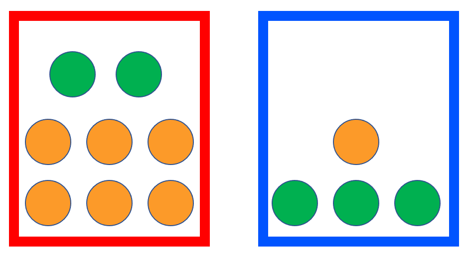
This example is a bit more complicated than the previous because there are two randomized actions involved here. The result of this action involves a combination of the color of the box and the type of fruits. Let’s start by considering the probability that the red box is drawn while an apple is picked up. Again, we can use the previous formula to calculate this probability. There are six numbers corresponding to the dice, and the number of fruits inside the red box is 8, so all the possibilities are \(6 \times 8\). But there are only numbers 1 through 4 and two apples, so there are only \(4 \times 2\) possibilities that qualify. So the probability is \[ \frac{4\times2}{6\times8} = \frac{4}{6} \times \frac{2}{8} = \frac{1}{6} \] It is easy to see that \(4/6\) is the probability of getting a number less than \(5\), i.e. the red box is selected. But what is the meaning of the second part, \(2/8\)? Since \(8\) is the number of fruits and \(2\) is the number of apples in the red box, it can be understood as the probability of getting an apple when the red box was selected. We refer to this probability as conditional probability and present it as \(\Pr(\text{Apple} | \text{Red}) = 2/8\). This discussion can be summarized as \[ \Pr ( \text{Red AND Apple} ) = \Pr( \text{Apple} | \text{Red} ) \Pr ( \text{Red} ) \] We can also easily get the probability of getting an apple under the other possibility, i.e. \[ \Pr(\text{Blue AND Apple}) = \Pr(\text{Apple} | \text{Blue} ) \Pr( \text{Blue} ) = \frac{3}{4} \times \frac{2}{6} = \frac{1}{4} \] “AND” corresponds to the “product rule”. \[ \Pr(E_1 \text{ AND } E_2) = \Pr(E_1 | E_2)\Pr(E_2) = \Pr(E_2 | E_1)\Pr(E_1) \] Going back to our original question, what is the probability of getting an apple? This random event can be labeled as “Red AND Apple OR Blue AND Apple”. Here, we have the second rule, i.e. “sum rule”, when considering the “OR” operator between two events that don’t happen simultaneously. \[ \Pr(E_1 \text{ OR } E_2) = \Pr(E_1) + \Pr(E_2) \]
Based on the sum rule, the probability of getting an apple is calculated as \[ \Pr( \text{Apple} ) = \Pr( \text{Red AND Apple} ) + \Pr( \text{Blue AND Apple} ) = \frac{5}{12} \]
Remark: we can compare it with the sum-product rule in permutation and combinations. When there are different types of solutions for one thing, the total number of possible solutions is the sum of the number of possible solutions for each type. When there are different steps in doing one thing, the total number of solutions is the product of the number of possible solutions in each step.
Similarly, you can verify the probabilities when orange is considered. If we use random variables to present the events, for example, the random variable \(X\) presents the box selected, \(1\) indicates red, and \(0\) indicates blue; the random variable \(Y\) presents the fruit drew, then the following table is called the joint distribution of two random variables.
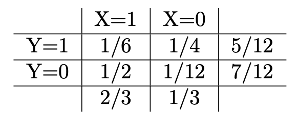
The last column is called the marginal distribution of random variable \(Y\), and the last row is the marginal distribution of random variable \(X\).
With the example above, the last interesting question is “What is the probability we chose the blue box if we get an orange?” First of all, it is a conditional probability, \(\Pr(X = 0 | Y = 0)\). According to the product rule, we know that this conditional probability is the ratio between \(\Pr(X=0 \text{ and } Y=0)\) and \(\Pr(Y=0)\). The first second has been calculated before and that is \(7/12\). Well, the first can be calculated by product rule again, i.e. \(\Pr( Y = 0 | X = 0 ) \Pr(X=0)\). Summarize, \[ \Pr(X = 0 | Y = 0) = \frac{\Pr( Y = 0 | X = 0 ) \Pr(X=0)}{\Pr(Y=0)} \]
\(\Pr(X=0|Y=0)\) is different from the conditional probability in the first question \(\Pr(Y=0|X=0)\). This probability is referred to as the posterior probability in the sense that we use the observation in the second step to update the probability of the first step. Correspondingly, the probability of drawing a blue box at the first step is called prior probability. The formula above is well known as Bayes formula.
From the joint distribution, the probability of drawing an apple \(\Pr(Y = 1)\) is \(5/12\). It is different from the probability of drawing an apple under the condition that the red box was selected, \(\Pr(Y=1 | X = 1) = 2/8\). This fact implies that the value of random variable \(Y\) depends on the value of \(X\), or random variable \(X\) and \(Y\) are dependent. If we add 1 apple and 11 oranges to the blue box, then \(\Pr(Y=1) = \Pr(Y=1 | X = 1)\). In this case, the value of random variable \(Y\) doesn’t depend on the value of \(X\), i.e. they are independent.
For two random variables \(X\) and \(Y\), we can use covariance to quantify the degree of association between two random variables. The covariance is defined as \[ \text{Cov}(X, Y) = \text{E}(X-\text{E}(X))(Y-\text{E}(Y)) \] The mean and variance of a weighted sum (linear combination) of two random variables are \[ \text{E}(aX+bY) = a\text{E}(X) + b\text{E}(Y) \] and \[ \text{Var}(aX+bY) = a^2\text{Var}(X) + 2ab\text{Cov}(X,Y) + b^2\text{Var}(Y) \] respectively.
Another characteristic value that quantifies the correlation between two variables is correlation. It is simply normalized covariance, i.e.
\[ \rho_{x,y} = \frac{\text{Cov}(X, Y)}{\sqrt{\text{Var}(X)} \cdot \sqrt{\text{Var}(Y)}} \] When the two variable uncorrelated, \(\text{Cov}(X, Y) = 0\), therefore \(\rho_{x,y} = 0\). Another two extreme cases are \(X = Y\), i.e. two random variables are the same, and \(X = -Y\). In these cases, \(\text{Cov}(X, \pm Y) = \pm \text{Cov}(X, X) = \pm \text{Var}(X)\), therefore, \(\rho_{x,y} = \pm 1\). Thus, different from covariance, the correlation is a number between \([-1, 1]\) due to the normalization. So, it is more comparable than covariance and people often use it to quantify the association between variables.
Next, we will consider a more challenging concept, continuous random variable. As you may notice, all the random events that we are considering can be represented by categorical outcomes. For example, flipping a coin has two outcomes, throwing a dice has 6 outcomes, and so on. For this kind of random event, it is sufficient to consider random variables only taking integer values. Thus we refer to the random variables discussed as discrete random variables. In practice, however, there are many other random events whose outcomes are not categorical but continuous values, for example, the temperature, the height of adult males, and so on. Therefore we need another type of random variable, a continuous variable.
Continuous random variables are not difficult to understand, they are nothing more than random variables that take real numbers, but the problem is how to describe their distribution. Again, let us abstract mathematical concepts from reality. Let’s consider such a background problem, assuming that I have height data for all boys in middle school in Sweden. Height is obviously not a categorical variable, but we can still use grouping to describe the distribution of height from a discrete perspective. Specifically, we can evenly divide the possible range of height into several groups, and then calculate the percentage of the number of people in each group to the total number of people. Yes, if you are familiar with basic statistics, you can tell that this is a histogram at a glance.
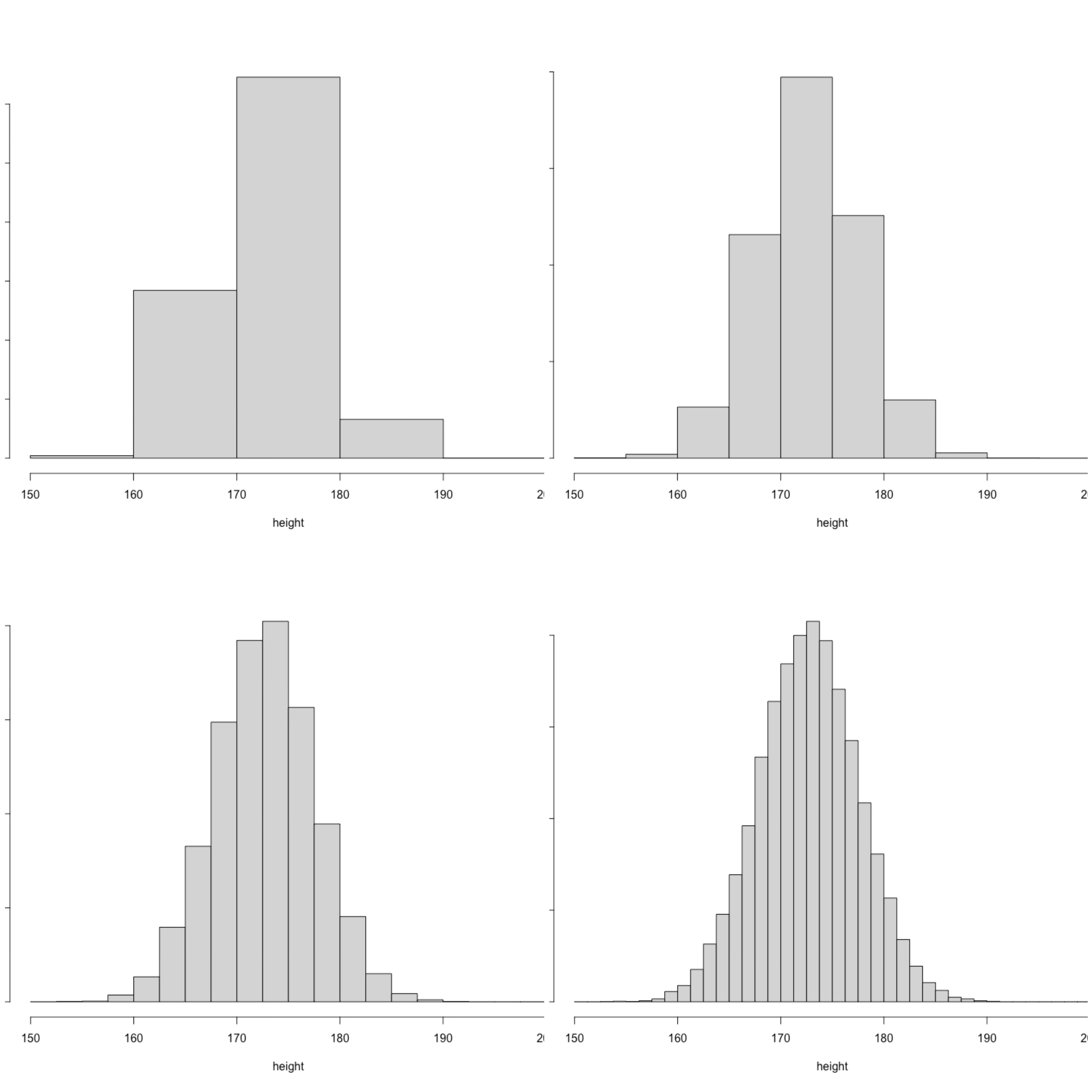
Such an approach has obvious flaws. For example, on the left-top of the plot, it is difficult for us to distinguish the probability of height being less than 175 and greater than 170 because these two values are combined into one group. How to do it? Very simple, we can split each large group into two small groups, of course, you also need to include more boys into the data set and then calculate the frequency of each group to represent the distribution of height, for example, on the right-top of the plot. If we still cannot distinguish the above probability, we can continue to split each group into two groups. Doing this we can see that the histogram is more detailed. If we have a sufficient large data set, we can continue to subdivide the height group and know the probability that we can distinguish the above two events. Suppose we put “all” the boys in middle school into this histogram, and each group can be subdivided infinitely. We can imagine that the upper edge of the histogram will be a smooth curve. We call this smooth curve the probability density function (p.d.f) and denote it as \(f(x)\). A valid p.d.f has to inherit two conditions from the p.m.f of a discrete random. First, the density value must be positive, \(f(x) > 0\), and the integral on the whole domain should be 1, \(\int_{-\infty}^{\infty} f(x) dx = 1\). With this function, we can calculate the probability of many events, as well as the expectation and variance. \[ \Pr(X<b) = \int_{-\infty}^bf(x)dx \] \[ \text{E}(X) = \int_{-\infty}^{\infty} xf(x) dx \]
One can compare the formula above with the expected value of a discrete random variable, \(\text{E}(X) = \sum_k k\Pr(x=k)\). You can see similar patterns, they all are the “sum” of all possible values times the corresponding probability or density values. Keep in mind that the integral symbol is an elongated S which indicates “sum”.
So far, we have only specified the basic conditions for a function to be a p.d.f , but the exact form of this function depends on the continuous distribution it represents. Next, we will learn about one of the most common continuous distributions: the Normal distribution.
A continuous random variable is Normally distributed, \(X \sim \mathcal{N}(\mu, \sigma^2)\), if its density function is
\[ f(x) = \frac{1}{\sigma \sqrt{2 \pi} } e^{- \frac{1}{2} \left( \frac{x-\mu}{\sigma}\right)^2 } \] The normal distribution is determined by two parameters, location parameter \(\mu\) and shape parameter \(\sigma^2\). Density functions of normal distribution with different parameters are displayed in the following picture.
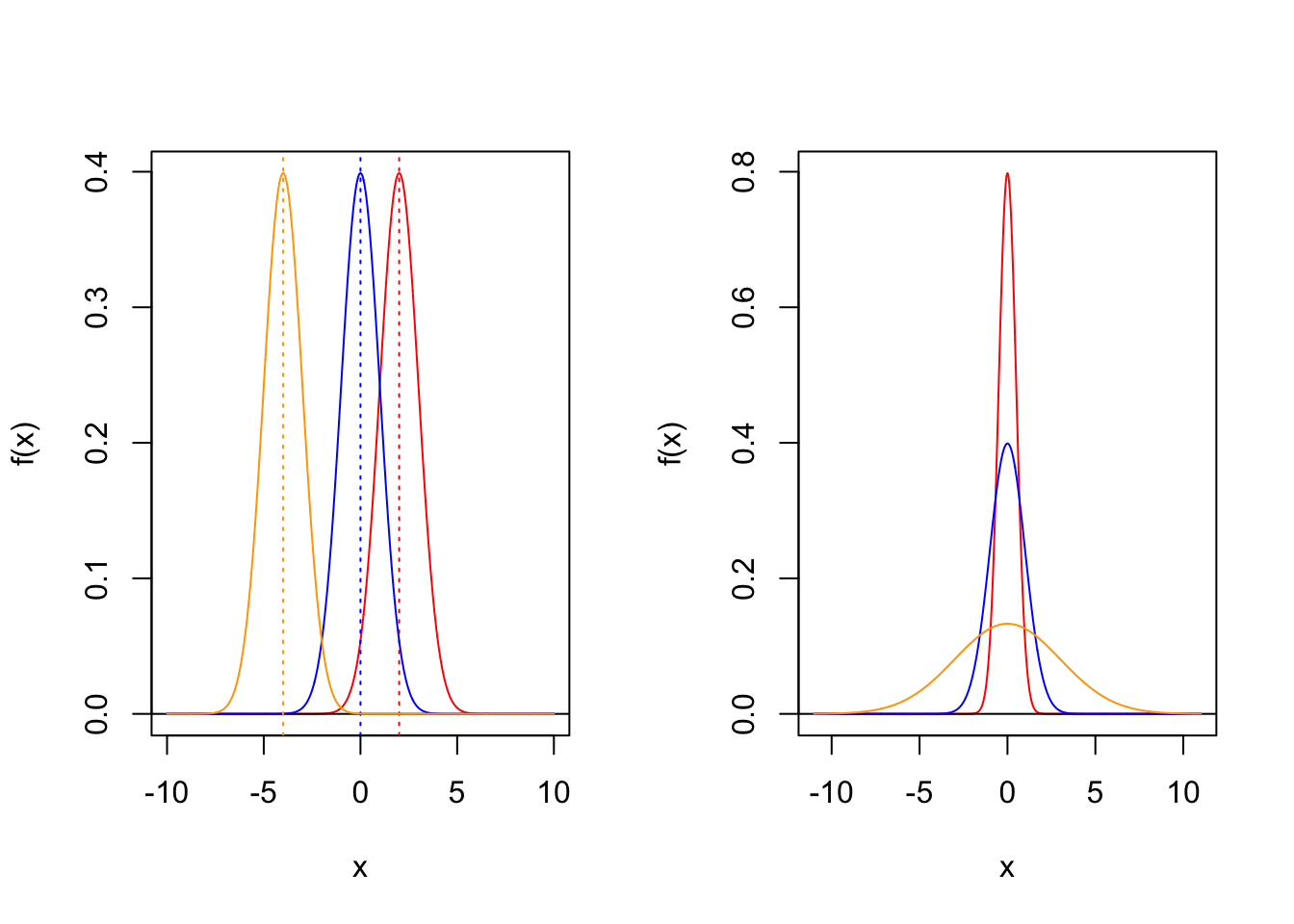
Now, I have two questions to you.
We have studied both discrete random variable and continuous random variable, their distribution of possible values can be presented by p.m.f and p.d.f respectively. The value of a p.m.f is just the probability when the random variable taking this value. However, what is the meaning of the value of a p.d.f?
What is the essence of the Normal distribution? In simpler terms, how would you introduce the concept of the Normal distribution to a middle school student?
Think about them and we will come back to them later on.
Likelihood analysis is an important concept in the modern statistics. A good understanding of likelihood can help you improve your knowledge in statistics. By understanding the relationship between likelihood and probability, you can build a bridge in statistical or data and probability modeling, allowing you to use models with greater confidence.
We have build up all the basic concepts of probability. In simple terms, probability is a mathematical model used to quantify the possibility of an event. The discussion of the possibility of this event is limited to the realm of rationality. For example, we can use probability to discuss the following questions.
“Imagine you are standing in the square in the city center of Umeå, close your eyes for 30 seconds, then open your eyes and catch the first man you see. How likely is his height above 180 cm?”
Let’s have a look at another scenario,
“You went to downtown last weekend. You stood in the square and closed your eyes, then after 30 seconds you opened your eyes and grabbed the man you saw first and measured his height. His height is 230 and you think it is unbelievable.”
In this case, we have a real observation of a random variable and want to evaluate the possibility of this observation. In this case, a proper word is likelihood value. I hope from the two examples above, you can see the difference between the two synonyms for “possibility.” In one word, likelihood value is the evaluation of the possibility to one observed valued, but probability evaluate the possibility of an event (somehow have not happened). Now, we can answer the first question above, what is the meaning of the value of a p.d.f? It present the likelihood of a real observation. For example, we may assume the height of adult men in Sweden is Normally distributed with mean 170 and SD 5.5 (I got these statistics from SCB, Statistiska centralbyrån), then the likelihood values of observing a man who is 179 and a men who is 230 are
So, it is almost impossible to see a men who is 230 in the center of Umeå city.
Remark 1: Unlike probability, likelihood is not standardized and is not a decimal between 0 and 1. When the standard deviation is very small, the likelihood value near the mean can be quite large. For example,
Remark 2 (HBG2K) : When people use the likelihood value, they often take the logarithm of it. One reason is that, even when the likelihood value is very small, we can still have a meaningful number for calculations. Another reason is that the distributions we commonly use, like the normal distribution, belong to the exponential family, so taking the logarithm transforms a nonlinear function into a linear one. For example,
Next, we summarize the facts about discrete random variable and continuous random variable in the following table.

You surely remember the previous question: what does the p.d.f of the normal distribution represent?
\[ f(x) = \frac{1}{\sigma \sqrt{2 \pi} } e^{- \frac{1}{2} \left( \frac{x-\mu}{\sigma}\right)^2 } \]
Or, to put it another way, just as the binary distribution aims to describe random events like coin tossing, what kind of random phenomenon is the normal distribution trying to describe?
Let’s start with en elementary understanding.
The normal distribution describes a bell-shaped, symmetric distribution of random phenomena, such as human IQ. Most people’s IQs are close to the mean, a smaller portion have higher or lower IQs, and only a very few have extremely high or low IQs. This forms a bell-shaped, symmetric distribution.
We can use more precise statistical terminology, such as confidence intervals, to describe this bell-shaped symmetric distribution of random phenomena. The normal distribution describes a random phenomenon where 68% of the probability is covered by the confidence interval of one SD around the mean, while the confidence interval of two SDs can cover 95% of the probability, and the confidence interval of three SDs can cover nearly all possibilities, as shown in the figure below.”
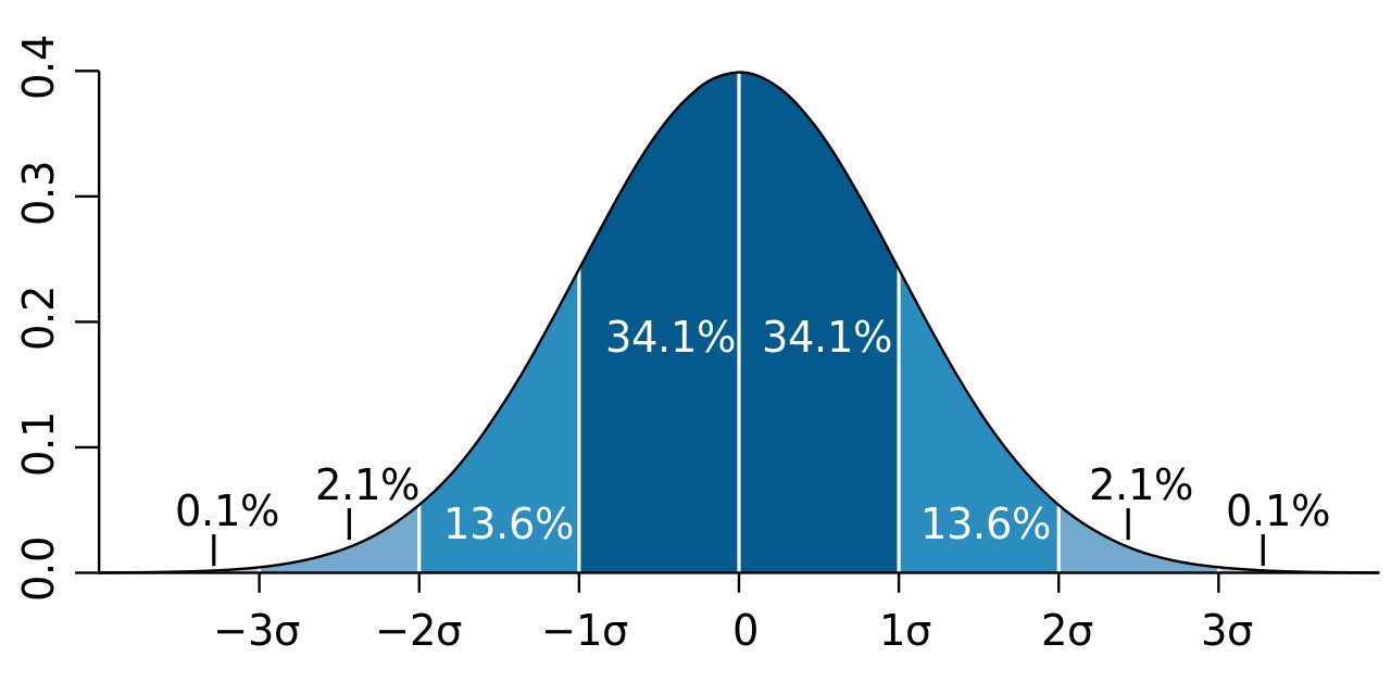
If you answer the question in such ways, then congratulations. You have rather good learning outputs from the previous basic statistics course. Next, let me introduce to you a deeper understanding based on the concept of likelihood. Let’s review the p.d.f of the normal distribution. Let’s watch an animation first.

Notice that \(\left(\frac{x-u}{\sigma}\right)^2\) is the normalized distance between an observation \(x\) and the center point \(\mu\). As mentioned before, the value of density function is the likelihood value of one observation, so the p.d.f is presenting the relationship between a specific observation \(x\) and its likelihood value. Then Normal distribution is describing such kind of random phenomenon:
The likelihood of an observation \(x_0\) is inversely proportion to the normalized distance between observed value \(x_0\) and the mean value \(\mu\).
More precisely, when the observed value is far from the center point, the likelihood of observing it will decrease rapidly, and this decrease is exponential, as displayed below.

In summary, the normal distribution essentially describes the relationship between the distance of observed values from the center point and likelihood within a class of random phenomena. It connects the geometric concept of distance with the statistical concept of likelihood.
With the likelihood idea, we can easily extend the normal distribution to a multidimensional case. In this note, I will just list several points help you to understand the main idea.
What is multidimensional case? For example, we may assume the height of Swedish adult men is normally distributed and denote as \(X_1 \sim \mathcal{N}(\mu_1, \sigma_1^2)\). We also know that another important physical indicator is weight, which can also be assumed to follow a normal distribution, denoted as \(X_2 \sim \mathcal{N}(\mu_2, \sigma_2^2)\). If, for each Swedish adult man, we simultaneously consider height and weight as descriptive features rather than just one or the other, then we enter a multidimensional scenario. So, what changes do we need to make in a multidimensional scenario? With the height-weight example,
We need two values to determine the location of the center point of the distribution, or we need a mean vector \((\mu_1, \mu_2)^{\top}\).
In the one dim case, we use variance/SD to control the shape of distribution. Naturally, we also need to consider the two variance simultaneously. However, this isn’t sufficient. We also need to take the association between the two variables, i.e. covariance, into account, as it is also an important factor in determine the overall shape. So, we need a covariance matrix to contain all the shape information, for example, in 2D case, \[ \left( \begin{matrix} \text{Var}(\text{Height}) & \text{Cov}(\text{Height}, \text{Weight}) \\ \text{Cov}(\text{Height}, \text{Weight}) & \text{Var}(\text{Weight}) \end{matrix} \right) \] Usually, a covariance matrix is denoted by \(\boldsymbol{\Sigma}\) which is a \(p \times p\) symmetric matrix (also need to be positive definite), \(p\) is the number of variables. In 2D case, the covariance matrix is usually presented as \[ \boldsymbol{\Sigma}= \left( \begin{matrix} \sigma_1^2 &\sigma_{12}\\ \sigma_{12} & \sigma_2^2 \end{matrix} \right) \] Given the definition of correlation, it is also can be represented as \[ \boldsymbol{\Sigma}= \left( \begin{matrix} \sigma_1^2 & \rho \sigma_1\sigma_2\\ \rho \sigma_1\sigma_2 & \sigma_2^2 \end{matrix} \right) \] where \(\rho\) is the correlation between \(X_1\) and \(X_2\)
We explained what is the essence of Normal distributions, that is likelihood value of an observation is inversely proportional to the normalized distance between the observation and mean value. Multivariate normal distribution should inherent this idea for sure. But the question is what is the normalized distance in 2D? Well, it is not such straightforward, I will explain it in another notes. (ToDo4Sia) We can just understand it as some normalized Euclidean distance in 2D. Thus, normal distributions, regardless of their dimensional, share a common pattern in their p.d.f , i.e. \[ f(\textbf{x}) \propto \exp ( - d_M(\textbf{x}, \boldsymbol{\mu}) ) \] where \(\textbf{x} = (x_1, x_2)^{\top}\), \(\boldsymbol{\mu} = (\mu_1, \mu_2)^{\top}\) and \(d_M(\cdot, \cdot )\) is the normalized distance between two input points. From the LHS of the formula, in in the 2D setting, the likelihood value of each observation (man) is determined by two inputs. From the RHS of the formula, the likelihood value is determined by the normalized distance \(d_M\), i.e. closer to the center point, higher possibility to observe.
Next, I show you some examples to demonstrate the arguments above.
Case 1: \(\sigma_1^2 = \sigma_2^2 = 1\) and \(\rho = 0\), i.e. the contrivance matrix is \[ \boldsymbol{\Sigma} = \left( \begin{matrix} 1 & 0 \\ 0 & 1 \end{matrix} \right) \]
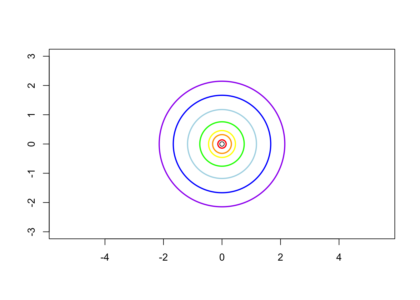
Case 2: \(\sigma_1^2 = 1\), \(\sigma_2^2 = 2\) and \(\rho = 0\) i.e. the contrivance matrix is \[ \boldsymbol{\Sigma} = \left( \begin{matrix} 1 & 0 \\ 0 & 2 \end{matrix} \right) \]
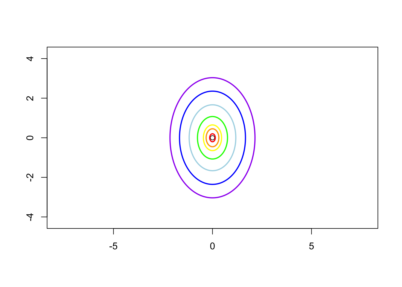
Case 3: \(\sigma_1 = 1\), \(\sigma_2 = 2\) and \(\rho = 0.8\), i.e. the contrivance matrix is \[ \boldsymbol{\Sigma} = \left( \begin{matrix} 1 & 1.13 \\ 1.13 & 2 \end{matrix} \right) \]
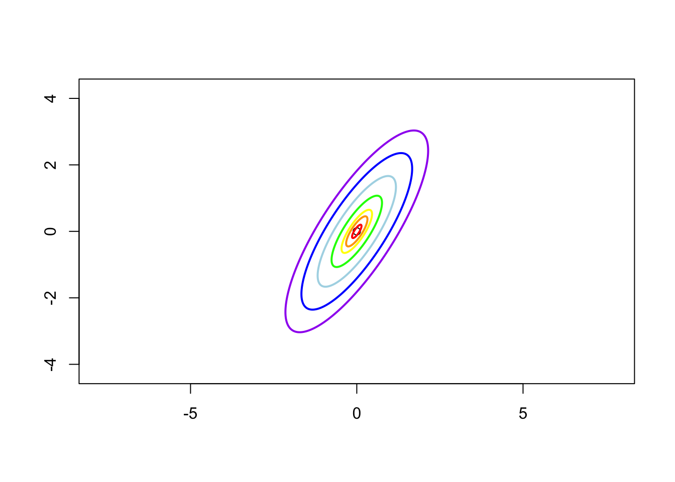
Case 4: \(\sigma_1 = 1\), \(\sigma_2 = 2\) and \(\rho = -0.8\), i.e. the contrivance matrix is \[ \boldsymbol{\Sigma} = \left( \begin{matrix} 1 & -1.13 \\ -1.13 & 2 \end{matrix} \right) \]
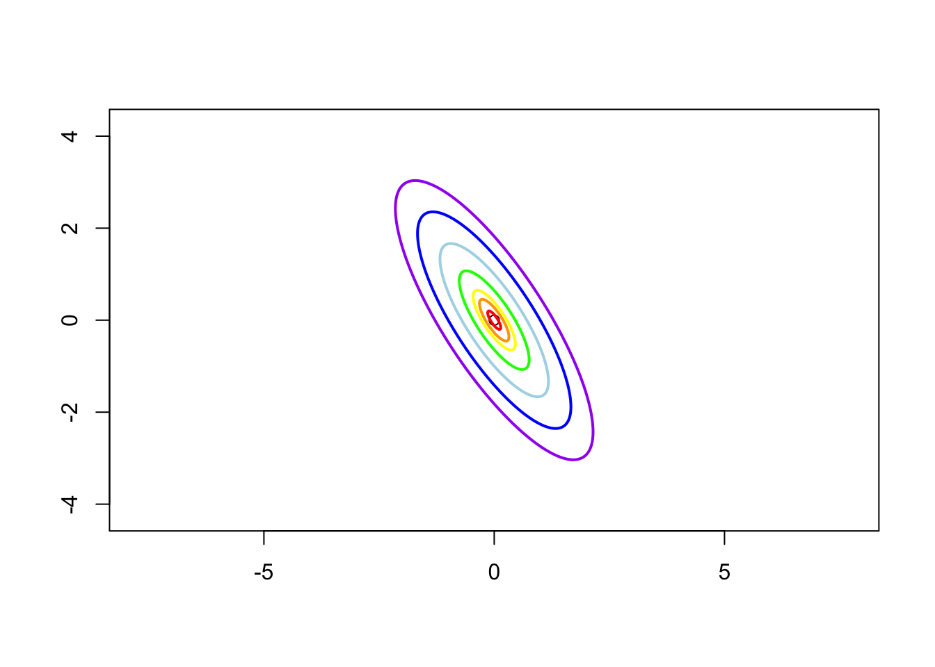
There are more stories about Normal (Gaussian) distribution. I will write a note about it. Please keep an eye on my space. ToDo4Sia: write a note telling the story of Gaussian distribution.
